


GENERATING TEST INPUTS FROM STRING CONSTRAINTS WITH AN AUTOMATA-BASED SOLVER
by
Marlin Roberts
A thesis submitted in partial fulfillment of the requirements for the degree of Master of Science in Computer Science Boise State University
August 2021
©2021
Marlin Roberts
ALL RIGHTS RESERVED
BOISE STATE UNIVERSITY GRADUATE COLLEGE
DEFENSE COMMITTEE AND FINAL READING APPROVALS
of the thesis submitted by
Marlin Roberts
Thesis Title: Generating Test Inputs from String Constraints with an Automata-Based Solver
Date of Final Oral Examination: 9th June 2021
The following individuals read and discussed the thesis submitted by student Marlin Roberts, and they evaluated the presentation and response to questions during the final oral examination. They found that the student passed the final oral examination.
Elena Sherman, Ph.D. Chair, Supervisory Committee
James Buffenbarger, Ph.D. Member, Supervisory Committee
Bogdan Dit, Ph.D. Member, Supervisory Committee
The final reading approval of the thesis was granted by Elena Sherman, Ph.D., Chair of the Supervisory Committee. The thesis was approved by the Graduate College.
ACKNOWLEDGMENTS
I would like to thank the faculty and staff of the Boise State University Com puter Science Department, whose professionalism and dedication made this pos-sible. I would like to thank my committee members, Dr. James Buffenbarger, and Dr. Bogdan Dit, for their support. Finally, a special acknowledgment for my advisor, Dr. Elena Sherman. She is an inspiration and shining example of “Excellence in Education.”
ABSTRACT
Software testing is an integral part of the software development process. To test certain parts of software, developers need to identify inputs that reach those parts. Data and control dependencies make this a non-trivial task, and as the complexity of software increases it becomes more difficult to manually derive such inputs. Due to complex data manipulations, this process is even more challenging for programs with string inputs, such as security applications. Thus, automated reach ability test input generation for string data types is an important research area.
Symbolic Execution is a path-sensitive static program analysis technique that can automatically generate conditions for inputs that reach a given program lo cation. Commonly, such conditions are encoded as automata that describe a set of strings at that location. Automata result from string operations applied to inputs
along that path. However, these automata do not necessarily correspond to string inputs that result in string values at the program location. To find those input values, we need to undo the effects of string operations through backward analysis. The intricate relationships between symbolic string values complicate this process. These relationships are due to non-injective string operations and data-flow dependencies of string values.
This thesis presents a novel method for test input generation for automata based string constraints. It uses single-track automata along with novel computational techniques to perform inverse string operations. Empirical evaluations on a set of benchmarks have shown this method to be effective in solving automata based string constraints from real-world applications.
TABLE OF CONTENTS
ABSTRACT……………………………………….
LIST OF TABLES…………………………………..
LIST OF FIGURES………………………………….
LIST OF ALGORITHMS……………………………..
LIST OF ABBREVIATIONS …………………………..
LIST OF SYMBOLS …………………………………
1 Introduction……………………………………..
1.1 Symbolic Execution . . . . . . . . . . . . . . . . . . . . . . . . . . . . . . . . . . . . . .
1.1.1 Symbolic Variables . . . . . . . . . . . . . . . . . . . . . . . . . . . . . . . . .
1.1.2 Symbolic Expressions . . . . . . . . . . . . . . . . . . . . . . . . . . . . . . .
1.1.3 Path Conditions . . . . . . . . . . . . . . . . . . . . . . . . . . . . . . . . . . .
1.1.4 Solving Integer Constraints. . . . . . . . . . . . . . . . . . . . . . . . . . .
1.1.5 Symbolic String Models . . . . . . . . . . . . . . . . . . . . . . . . . . . . .
1.1.6 Symbolic String Operations . . . . . . . . . . . . . . . . . . . . . . . . . .
1.1.7 String Predicates. . . . . . . . . . . . . . . . . . . . . . . . . . . . . . . . . . .
1.1.8 Solving String Constraints . . . . . . . . . . . . . . . . . . . . . . . . . . .
1.1.9 Inverse String Operations . . . . . . . . . . . . . . . . . . . . . . . . . . . .
1.2 Motivating Example. . . . . . . . . . . . . . . . . . . . . . . . . . . . . . . . . . . . . .
1.3 Challenges . . . . . . . . . . . . . . . . . . . . . . . . . . . . . . . . . . . . . . . . . . . . .
1.4 Solver Characteristics. . . . . . . . . . . . . . . . . . . . . . . . . . . . . . . . . . . . .
1.5 Thesis Statement . . . . . . . . . . . . . . . . . . . . . . . . . . . . . . . . . . . . . . . .
2 Background and Related Work ……………………….
2.1 String Models. . . . . . . . . . . . . . . . . . . . . . . . . . . . . . . . . . . . . . . . . . .
2.2 Solvers . . . . . . . . . . . . . . . . . . . . . . . . . . . . . . . . . . . . . . . . . . . . . . . .
2.3 Constraint Solving . . . . . . . . . . . . . . . . . . . . . . . . . . . . . . . . . . . . . . .
3 Approach……………………………………….
3.1 Backward Analysis . . . . . . . . . . . . . . . . . . . . . . . . . . . . . . . . . . . . . . .
3.1.1 Constraint Graph . . . . . . . . . . . . . . . . . . . . . . . . . . . . . . . . . .
3.1.2 Transposed Constraint Graph. . . . . . . . . . . . . . . . . . . . . . . . .
3.1.3 Graph Traversal . . . . . . . . . . . . . . . . . . . . . . . . . . . . . . . . . . .
3.1.4 Fallback Sequence . . . . . . . . . . . . . . . . . . . . . . . . . . . . . . . . . .
3.1.5 Node Evaluation . . . . . . . . . . . . . . . . . . . . . . . . . . . . . . . . . . .
3.1.6 Sound and Complete Operations. . . . . . . . . . . . . . . . . . . . . . .
3.1.7 Handling Over-Approximation . . . . . . . . . . . . . . . . . . . . . . . .
3.1.8 Maintaining Related Values . . . . . . . . . . . . . . . . . . . . . . . . . .
3.1.9 Termination . . . . . . . . . . . . . . . . . . . . . . . . . . . . . . . . . . . . . .
3.1.10 Complexity . . . . . . . . . . . . . . . . . . . . . . . . . . . . . . . . . . . . . . .
3.1.11 Limitations . . . . . . . . . . . . . . . . . . . . . . . . . . . . . . . . . . . . . . .
3.2 Inverse String Operations. . . . . . . . . . . . . . . . . . . . . . . . . . . . . . . . . .
3.2.1 Formal Definitions and Algorithms . . . . . . . . . . . . . . . . . . . . .
4 Implementation…………………………………..
4.1 Inverse String Operation Classes . . . . . . . . . . . . . . . . . . . . . . . . . . . .
4.2 Solver . . . . . . . . . . . . . . . . . . . . . . . . . . . . . . . . . . . . . . . . . . . . . . . . .
4.3 Integration with Symbolic Pathfinder. . . . . . . . . . . . . . . . . . . . . . . . .
5 Evaluation ………………………………………
5.1 Correctness. . . . . . . . . . . . . . . . . . . . . . . . . . . . . . . . . . . . . . . . . . . . .
5.1.1 Correctness Results. . . . . . . . . . . . . . . . . . . . . . . . . . . . . . . . .
5.2 Practicality. . . . . . . . . . . . . . . . . . . . . . . . . . . . . . . . . . . . . . . . . . . . .
5.2.1 Results . . . . . . . . . . . . . . . . . . . . . . . . . . . . . . . . . . . . . . . . . .
5.3 Scalability. . . . . . . . . . . . . . . . . . . . . . . . . . . . . . . . . . . . . . . . . . . . . .
5.4 Validity. . . . . . . . . . . . . . . . . . . . . . . . . . . . . . . . . . . . . . . . . . . . . . . .
5.5 Summary . . . . . . . . . . . . . . . . . . . . . . . . . . . . . . . . . . . . . . . . . . . . . .
6 Conclusion………………………………………
REFERENCES……………………………………..
LIST OF TABLES
2.1 Popular String Constraint Solvers . . . . . . . . . . . . . . . . . . . . . . . . . . .
4.1 Metrics for Initial and Current Code base. . . . . . . . . . . . . . . . . . . . . .
4.2 Major Dependencies . . . . . . . . . . . . . . . . . . . . . . . . . . . . . . . . . . . . . .
4.3 String and Inverse String Operations . . . . . . . . . . . . . . . . . . . . . . . . .
5.1 Test Case Properties. . . . . . . . . . . . . . . . . . . . . . . . . . . . . . . . . . . . . .
5.2 Correctness Results . . . . . . . . . . . . . . . . . . . . . . . . . . . . . . . . . . . . . .
5.3 Benchmark Properties . . . . . . . . . . . . . . . . . . . . . . . . . . . . . . . . . . . .
5.4 Benchmark Timing Ratios-Series One . . . . . . . . . . . . . . . . . . . . . . .
5.5 Benchmark Timings-Series Two. . . . . . . . . . . . . . . . . . . . . . . . . . . .
5.6 Benchmark Timings-Series Three. . . . . . . . . . . . . . . . . . . . . . . . . . .
5.7 Effect of Alphabet Size on Test Case 10 ab. . . . . . . . . . . . . . . . . . . . .
LIST OF FIGURES
1.1 Symbolic Execution with Integer Inputs. . . . . . . . . . . . . . . . . . . . . . .
1.2 Symbolic Execution with String Input . . . . . . . . . . . . . . . . . . . . . . . .
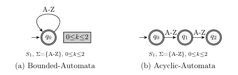
1.3 Bounded vs. Acyclic Automata, sum of={A-Z},0 k 2 . . . . . . . . . .
1.4 Acyclic Automata for Concrete and Symbolic String Variables S 1,S 2
1.5 Removal of Concrete String from Concatenation Result. . . . . . . . . . .
1.6 Motivating Example,Concatenation of Symbolic Strings. . . . . . . . . .
1.7 Concatenation of Symbolic Strings and Application of Predicate. . . .
1.8 Attempting to Determine S1, S2 with Sub string Operation . . . . . . . .
2.1 Simple Finite State Automata . . . . . . . . . . . . . . . . . . . . . . . . . . . . . .
2.2 Bounded vs. Acyclic-Automata . . . . . . . . . . . . . . . . . . . . . . . . . . . . .
2.3 Over-Approximation with Unbounded-Automata. . . . . . . . . . . . . . . .
2.4 Avoiding Over-Approximation with Acyclic-Automata. . . . . . . . . . . .
2.5 Related Inputs . . . . . . . . . . . . . . . . . . . . . . . . . . . . . . . . . . . . . . . . . .
3.1 Constraint Graph. . . . . . . . . . . . . . . . . . . . . . . . . . . . . . . . . . . . . . . .
3.2 Transposed Constraint Graph . . . . . . . . . . . . . . . . . . . . . . . . . . . . . .
3.3 Inverse Node with Solution Set . . . . . . . . . . . . . . . . . . . . . . . . . . . . .
3.4 Input Nodes and Solution Sets. . . . . . . . . . . . . . . . . . . . . . . . . . . . . .
3.5 Sound and Complete Inverse Operation. . . . . . . . . . . . . . . . . . . . . . .
3.6 Hand ling Over-Approximation . . . . . . . . . . . . . . . . . . . . . . . . . . . . . .
3.7 Handling Related Inputs. . . . . . . . . . . . . . . . . . . . . . . . . . . . . . . . . . .
4.1 Input Generator Components. . . . . . . . . . . . . . . . . . . . . . . . . . . . . . .
4.2 Symbolic Pathfinder Data Flow. . . . . . . . . . . . . . . . . . . . . . . . . . . . .
4.3 Example SPF Input and Output . . . . . . . . . . . . . . . . . . . . . . . . . . . .
4.4 Test Case Constraint Graph. . . . . . . . . . . . . . . . . . . . . . . . . . . . . . . .
5.1 Non-Injective and Unsound Operations Test Case Code . . . . . . . . . .
5.2 Non-Injective and Unsound Operations Constraint Graph. . . . . . . . .
5.3 Multiple Outgoing Edges Test Case Code . . . . . . . . . . . . . . . . . . . . .
5.4 Multiple Outgoing Edges Constraint Graph. . . . . . . . . . . . . . . . . . . .
5.5 Multiple Inputs Test Case Code. . . . . . . . . . . . . . . . . . . . . . . . . . . . .
5.6 Multiple Inputs Constraint Graph . . . . . . . . . . . . . . . . . . . . . . . . . . .
5.7 Test Flow. . . . . . . . . . . . . . . . . . . . . . . . . . . . . . . . . . . . . . . . . . . . . .
5.8 Related Unsound Operations Test Code. . . . . . . . . . . . . . . . . . . . . . .
5.9 Related Unsound Operations Constraint Graph. . . . . . . . . . . . . . . . .
5.10 Box Plot of Series One Runtime Ratio. . . . . . . . . . . . . . . . . . . . . . . .
5.11 Box Plot of Series Two Run times . . . . . . . . . . . . . . . . . . . . . . . . . . . .
5.12 Box Plot of Series Three Run times. . . . . . . . . . . . . . . . . . . . . . . . . . .
5.13 Growth in Runtime of Selected Test Cases. . . . . . . . . . . . . . . . . . . . .
LIST OF ALGORITHMS
1 Traverse Function. . . . . . . . . . . . . . . . . . . . . . . . . . . . . . . . . . . . . . . .
2 Evaluate Function for Predicate Nodes . . . . . . . . . . . . . . . . . . . . . . .
3 Evaluate Function for Input Nodes. . . . . . . . . . . . . . . . . . . . . . . . . . .
4 Evaluate for Sound and Complete Inverse Operations . . . . . . . . . . . .
5 Evaluate for Over-Approximating Inverse Operations . . . . . . . . . . . .
6 Evaluate Function for Related Value Operations . . . . . . . . . . . . . . . .
7 Algorithm for in v Con cat() . . . . . . . . . . . . . . . . . . . . . . . . . . . . . . .
8 Algorithm for in v Delete(). . . . . . . . . . . . . . . . . . . . . . . . . . . . . . . .
9 Algorithm for in v Delete Char At() . . . . . . . . . . . . . . . . . . . . . . . .
10 Algorithm for in v Insert() . . . . . . . . . . . . . . . . . . . . . . . . . . . . . . . .
11 Algorithm for in v Replace(). . . . . . . . . . . . . . . . . . . . . . . . . . . . . . .
12 Algorithm for in v Reverse(). . . . . . . . . . . . . . . . . . . . . . . . . . . . . . .
13 Algorithm for in v To Lower Case() . . . . . . . . . . . . . . . . . . . . . . . . .
14 Algorithm for in v To Upper Case(). . . . . . . . . . . . . . . . . . . . . . . . . .
15 Algorithm for in v Sub string(start,end) . . . . . . . . . . . . . . . . . . .
16 Algorithm for in v Sub string(start) . . . . . . . . . . . . . . . . . . . . . . . .
17 Algorithm for in v Trim(). . . . . . . . . . . . . . . . . . . . . . . . . . . . . . . . . .
LIST OF ABBREVIATIONS
SPF– Symbolic Pathfinder
SE– Symbolic Execution
PC– Path Conditions
SAT– Satisfiable
UNSAT– Unsatisfiable
F S A– Finite State Automata
S MT–Satisfiability Modulo Theory
TCG–Transposed Constraint Graph
LIST OF SYMBOLS
A Finite State Automata
L(A) Language of Finite State Automata
Alphabet of Finite State Automata
k Length of String Accepted by Finite State Automata
Empty String
SECTION 1
INTRODUCTION
Once relegated to a brief ad-hoc effort, software testing has become a well-established systematic software development process. Primary factors driving the adoption of testing are the increased cost of software defects that can cause security breaches and failures of safety critical systems. As software testing became an integral part of software development, software bacame more complex with intricate data and control dependencies. This has caused an increase in the test case generation effort, and in-particular identifying test cases that reach specific locations in code. With simpler software it was feasible for a programmer to reason about test inputs that reach program locations, however with complex software the programmers require automated approaches to aid in generating test inputs for code reachability.
In response to these challenges, researchers leverage static program analysis techniques such as Symbolic Execution (SE) [5,12] to generate test inputs [5,7,17], detect security vulnerabilities, and find program defects. When used to generate inputs, SE helps with finding a feasible path to the targeted location, which needs to be executed by a test. However, it remains difficult to analyze and generate test cases for programs that manipulate variables of complex data types such as strings, and have variables entangled in non-trivial computations.
This work investigates approaches that improve test input generation for Java String manipulating programs using SE techniques. Before explaining challenges that this work addresses, the next section details the SE approach to test input generation for Java string programs. It starts with an overview of SE testing and continues with modeling sets of strings as automata.
1.1 Symbolic Execution
SE is a path-sensitive static program analysis technique that simulates the ex ecution of a program on symbolic inputs. In general, the process consists of interpreting the code to determine the values that variables may take and deter mining the condition (or constraint) that defines a path. To use it as a white-box test case generator, a SE engine sends that constraint to a solver and asks to return a satisfiable solution. An overview of the process follows, starting with the introduction of symbolic variables.
1.1.1 Symbolic Variables
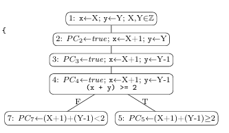
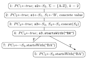
Figures 1.1 and 1.2 present examples of SE on Java methods with integer and string inputs, respectively. SE treats program input variables as symbolic values by using Symbolic Variables to represent all possible concrete values that a program input variable may take. Figure 1.1b shows the assignment of symbolic variables to integer arguments x and y at the top of the symbolic execution tree: (x X) and (y Y). Figure 1.2b shows similar assignments for strings s 1, s 2 and s 3.
1 public void intEx (int x, int y) {
2 x = x + 1;
x = x + 1;
3 y = y- 1;
4 if ((x + y) >= 2 ) {
5 // true branch
6 } else {
7 // false branch
8 }
9 }

(a) Method with integer inputs (b) Symbolic Execution Tree
Figure 1.1: Symbolic Execution with Integer Inputs
1 public void strEx (String s2) { 2 String s1 = “B”; 3 String s3 = s1.concat(s2);
4 if (s3.startsWith(“BA”)) { 5 // true branch 6} else {
7 // false branch
8}
9}

(a) Method with string input (b) Symbolic Execution Tree
Figure 1.2: Symbolic Execution with String Input
1.1.2 Symbolic Expressions
When SE encounters Domain Operations, such as integer addition or string con catenation, it creates new Symbolic Expressions by applying those operations to symbolic variables or existing symbolic expressions. The program statement on line 2 of Figure 1.1a, (x = x + 1), results in the symbolic expression and assignment (x X+1) shown in Figure 1.1b. String concatenation on line 3 of Figure 1.2a produces the symbolic expressions on line 3 o 1.2b.
1.1.3 Path Conditions
SE maintains a propositional symbolic formula known as the Path Condition (PC). The PC represents the constraints that must be satisfied to execute the path followed by SE. The PC is a conjunction of symbolic predicates, and initially set to true: PCn true, where n is a program location. When evaluating a conditional statement, SE conjoins a symbolic predicate to the PC based on the conditional expression, branch taken and current symbolic state. Figure 1.1b shows the results of evaluating the statement (if ((x + y) >= 2)) with (x X+1) and (y Y 1). Thetrue branch PC is (PC5 true ((X+1)+(Y 1)) 2)) and the false branch PC is (PC7
true ((X + 1) + (Y 1)) < 2)). The initial true value is eliminated from the PC when it is simplified. The evaluation of the statement on line 4 of Figure 1.2a produces (PC5 S3.startsWith(“BA”)) and (PC7 S3.startsWith(“BA”)) for true and false, respectively (where is the negation symbol).
1.1.4 Solving Integer Constraints
Once a PC is constructed, SE uses a Constraint Solver, or simply Solver, to determine:
• Whether a PC evaluates to true (the PC is satisfiable, or SAT) or false (the PC is unsatisfiable, or UNSAT). A PC is SAT if there is a solution that evaluates its formula to true, otherwise it is UNSAT. A SAT PC means that the path explored by SE is feasible (or reachable). Note that this type of analysis determines if constraints can be satisfied and does not necessarily f ind satisfiable assignments.
• If there are satisfiable assignments of variables in the PC that correspond to the concrete input values that execute that program path. This is the basis of test input generation using SE
In order to produce a solution for the true branch (PC5) in the example given in Figure 1.1, the solver must solve the inequality ((X + 1) + (Y 1)) 2) for the symbolic variables X and Y. For X, subtracting (Y 1) from both sides of
the inequality yields ((X +1) 2 (Y 1)). Since X was modified by a domain operation (addition), the solver performs the inverse operation (subtraction) in order to isolate X: ((X+1) 1 2 (Y 1) 1), whichsimplifies to (X 2 Y). If the inequalities for X and Y cannot be solved, the PC for that branch becomes UNSAT and the path is marked as infeasible, otherwise it is SAT. The inequalities in this example can be satisfied with X = 1, Y = 1. When using these values as inputs for x and y, the program executes the true branch.
Solving integer constraints systematically is possible because the inverses of integer operations are well defined. Addition and subtraction have an inverse relationship as do multiplication and division. Clearly, the algebra for solving integer inequalities is well established. However, the theory of strings is not as well developed and cannot guarantee for string operations to have inverses. Thus, making it difficult to design generic algorithms for solving string constraints. Before examining the problems related to automata-based string constraint solving, the automata-based string model is introduced.
1.1.5 Symbolic String Models
A Symbolic String Model (or simply String Model) is the construct used to model a set of strings. Since the number of possible values a symbolic string can take grows exponentially with length, storing these values as a set of concrete strings is not feasible. While Section 2.1 presents a detailed comparison of constructs used to
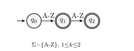
model strings, two types of automata commonly used for this purpose are discussed here: bounded and acyclic. Figure 1.3 presents a comparison of bounded and acyclic automatons for a string sum of = {A-Z}, 0 k 2. The bounded-automaton in Figure 1.3a is more compact, because it tracks the string length separate from the automaton. The acyclic-automata enforces string length by construction. Previous research on evaluating automata types for modeling strings in SE has shown that acyclic-automata reduce over-approximation (discussed in Section 1.4) in string operations [16]. Since accuracy is essential to the efficiency of test case generation, this work focuses on the acyclic-automata model. From this point on, references to automata assume acyclic-automata, and all references to string models assume acyclic-automata string models.

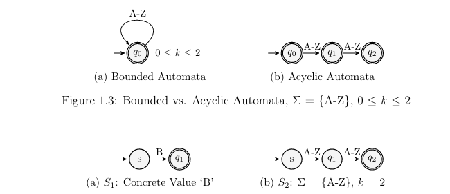
As further examples of acyclic models, Figure 1.4 shows acyclic-automata models for strings S1 and S2. Figure 1.4a shows S1 with the single (or concrete) value “B”. Figure 1.4b shows S2 of length (k) = 2 and alphabet ( ) = {A Z}. The example shown in Figure 1.2 uses strings S1 and S2 as defined in Figure 1.4. The next subsection explains string operations.
1.1.6 Symbolic String Operations
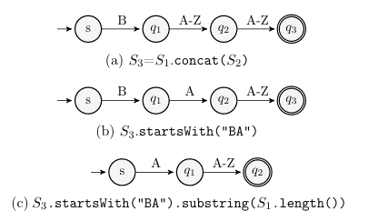
The example in Figure 1.2 includes concatenation of S1 and S2. Since S1 and S2 can represent more than one string value, the result of this operation is the cross product of the sets S1 and S2. For example, if strings prefix = {a, b} and suffix = {c, d}, prefix.concat(suffix) results in the strings {ac, ad, bc, bd}. Figure 1.5a shows the result of S1.concat(S2), which is assigned to S3. It is important to note that while the automaton in Figure 1.5a represents all possible values of string S3 at that location, the automaton cannot distinguish between the “B” and string S2:
it has aggregated the states and transitions. Next, SE encounters a conditional statement at line 4 and applies the predicate to determine the PC for each branch

1.1.7 String Predicates
The predicate in the conditional statement at line 4 of Figure 1.2 is the Java string method startsWith(“BA”) applied to string S3. Post-predicate string values for S3 in the true branch all start with “BA”, with all other pre-predicate string values executing the false branch. Figure 1.5b shows the automaton for S3 on the true branch. Note that all possible values for S3 on the true branch fail to execute the true branch if used as input values: The string “B” concatenated with strings that begin with “BA” results in strings that start with “BB”, which execute the false branch instead.
1.1.8 Solving String Constraints
When SE determines a symbolic expression for a string, it performs the string operations to determine possible values of the program variable at that location. At conditional statements, SE applies the predicate to restrict these values and determine if a branch is feasible. If there are possible values, then the PC for that branch is UNSAT, which means that the branch cannot be executed on that path. Even though SE generates possible values for strings taking a branch, those values cannot serve as inputs reaching that branch, because string operations applied to inputs modify their initial values. These string operations must be “undone,” i.e., “inverted” in order to generate inputs from string values at the branch outcome.
1.1.9 Inverse String Operations
To generate values for S2 that execute the true branch, the concatenation must be “undone” with Inverse String Operations. An inverse string operation has an inverse relationship with a corresponding string operation. For example, a string operation that inserts a character at an index can be “inverted” with one that deletes the character at that index. Inverse string operations may be defined in terms of existing string operations, as + and
for integers, or may require custom algorithms that modify the string model elements. This work assumes that all string operations of the string constraint solver are available for defining inverse string operations.
Note that when referring to a Java string method specifically, the term method is used. The text uses the term operations when it refers to a string operation on an automaton. The string operations model the Java string methods, and have corresponding inverse string operations.
In the example given in Figure 1.5, it is possible to define inverse concatenation using the Java string method substring(int start), which returns the substring from index start to the end of the string. Since S1 a concrete value, it has a single length which can be referenced with S1.length(). Combining these methods yields S2 = S3.substring(S1.length()). Figure 1.5c shows the result: an automaton that accepts strings of length 2 which start with “A”. This auomaton accepts all strings that make s2 successfully reach the true branch.
1.2 Motivating Example
In the previous string example, two factors facilitate the straightforward imple
mentation of the inverse concatenation:
The solver can determine the length of S1- Since S1 is concrete with a known length (1), the solver removes the correct number of characters from S3 to find S2.
The inverse operation is expressed in terms of an existing string operation- This eliminates the need to design new operations.
However, making minor changes to the previous string example significantly increases the complexity of the string constraint. Figure 1.6 presents this example, with the following modifications:
The concatenation arguments are both symbolic string inputs- The inputs (s1 S1), (s2 S2) are defined = {A-Z} and 1 k 2. Now the solver must account for ranges of input lengths.
The predicate is now contains(“BAA”)- Applying this predicate to the concate nation result creates a complex automaton with several accepting paths.
The goal is to compute values for inputs s1 and s2 that reach the true branch of the conditional statement at line
PC4 S3.contains(“BAA”). Figure 1.7 shows S1 and S2, each contributing either 1 3. The PC for this branch is
PC4 S3.contains(“BAA”). Figure 1.7 shows S1 and S2, each contributing either 1 or 2 characters to the concatenated result which is the automaton with length 2less than k less than 4 shown in Figure 1.7b. Figure 1.7c shows the result of applying predicate contains(“BAA”). Since a minimum of 3 characters in a string are required to make the predicate evaluate
1 public void strEx (String s1, String s2) {
2 String s3 = s1.concat(s2);
3 if (s3.contains(“BAA”)) {
4 // true branch
5 } else {
6// false branch
7}
8 }
(a) Method with string inputs
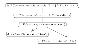

(b) Symbolic Execution Tree
Figure 1.6: Motivating Example, Concatenation of Symbolic Strings
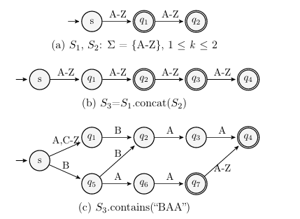

(c) S3.contains(“BAA”)
Figure 1.7: Concatenation of Symbolic Strings and Application of Predicate
to true, the result has a range of lengths: 3less than kless than 4. In this example, designing an inverse conatenation is complicated by the following factors: S1 and S2 represent strings of various lengths- The inverse concatenation needs to account for 4 combinations of lengths of S1 and S2: (S1: k = 1, S2: k = 1),
(S1: k = 1, S2: k = 2), (S1: k = 2, S2: k = 1), (S1: k = 2, S2: k = 2)
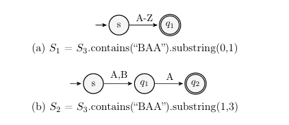
Using substring operation as inverse for concat introduces spurious strings- The substring operation in the previous example produces a solution containing only strings that execute the target path. An over-approximating inverse operation introduces Spurious strings that do not execute the desired path. Using the substring operation as before with the same lengths (S1: k = 1, S2: k = 2) results in spurious strings. In this case both the starting and ending indexes of the desired substrings are specified: (S1 = S3.contains(“BAA”).substring(0,1)) and (S2 = S3.contains(“BAA”).substring(1,3)). The result for S1 in Figure 1.8a accepts “A” and the result for S2 in Figure 1.8b accepts “AA”. However, using s1 = “A”, s2 = “AA” does not execute the desired path. While this solution does contain the single correct result for lengths (S1: k = 1, S2: k = 2), (s1 = “B” and s2 = “AA”), it also contains 51 spurious combinations.

The resulting automaton lost information about S1 and S2- Due to inability to determine which states and transitions correspond to each target and argument, programming a new precise inverse operation to separate them is difficult. S1 and S2 are dependent- The concatenation of S1 and S2 introduces dependencies between their values in that choosing a test input value for one may affect valid choices for the other. Choosing values for independent variables can be done without regard for other variables.
1.3 Challenges
These specific problems of generating test inputs for string manipulating programs can be categorized into the following challenges. Modeling Inverse String Operations- Some inverse string operations can be defined in terms of existing automata string operations. An example of an in verse relationship between Java methods are insert(int offset, char c) and delete(int start, int end). In this case, the delete method can be used as the
inverse of the insert method. Since the solver knows the length (1) and the position (offset) of the inserted element, it can call delete(offset, (offset + 1)) to invert the insert operation. However, the method insert(int offset, String str) cannot be modeled with existing operations. If the argument str represents a single string value, such as “AB”, then the length can be determined and we can model the inverse operation with delete(int start, int end). This is because we know about the position and length of the argument. If the argument str is not concrete, but instead represents string values of more than one length, this naive approach fails. Thus, new inverse operations should be provided. Handling Non-Injective Functions- Some string operations are non-injective, meaning they do not have a 1:1 relationship between each input and output. An example of a non-injective function is the method delete(int start, int end). To invert the delete operation, the solver can determine the location and length of the deleted characters, but cannot determine what was deleted. Performing the delete operation on multiple unique strings may produce the same output, hence making it impossible to determine the relation between the result and the original strings of the delete operation. Maintaining Dependencies and Relationships- Reaching a given point during execution may depend on the values and relationships of multiple variables. All of them must be solved and relationships between the values maintained. An input can be used in different locations, or be related to itself such as a string being concatenated with itself. Before presenting the thesis statement, it is important to define solver character istics and how they contextualize computed solutions.
1.4 Solver Characteristics
Asound constraint solver does not report a PC is UNSAT when it is SAT. In other words, if a PC has a solution, a sound solver finds it, i.e., it does not report any false negatives. However, a sound solver may report an UNSAT PC as being SAT, termed a false positive, due to Over-approximation of the solution set in order to make operations closed. Over-approximation occurs when a solution contains all concrete values that satisfy a PC, as well as some that do not. A complete solver never reports an UNSAT PC as SAT. In other words, if a PC has no solution, a complete solver never reports one. It can also be said that a complete solver never reports false positives. However, a complete solver may miss a solution and report a SAT PC as UNSAT, a false negative. This is Under-approximation, which occurs when a solution contains only values that satisfy a PC but contains a subset of all such values.
Some amount of over-approximation (false positives) can be tolerated, and some string constraint solvers allow for over-approximation in order to ensure a sound solution [19]. These approaches may produce a solution such as the one presented in Figure 1.8 since it does produce the valid combination of inputs for the chosen lengths (S1 = “B”, S2 = “AA”). However, that is the only valid combination out of the 52 possible, which is a considerable number of false positives.
In general, it is impossible for a solver to be both sound and complete for undecidable problems such as the satisfiability of a string PC [3]. The focus of this work is to demonstrate practical methods that can produce sound and complete solutions within certain contexts, such as within the length of input strings.
1.5 Thesis Statement
A complete test input generator for Java string programs can be implemented using symbolic execution with an acyclic-automata based string constraint solver that accurately models inverse string operations and ensures consistency between dependent solutions.
This work aims to address the following research questions that support this statement:
• RQ1
Can all inverse string operations be accurately modeled? In answer- ing this question we investigate over approximation and the use of existing string operations, as well as methods for implementing those that cannot be modeled with existing string operations.
• RQ2
How to maintain the dependencies while solving for inputs? Since single-track automata cannot model relationships between strings, we investigate techniques to maintain these relationships.
• RQ3
Is the solution practical and effective? We evaluate whether the meth
ods can be used with real-world programs and their effectiveness at finding
test inputs.
This rest of this thesis is organized as follows: Section 2 introduces string models, constraints and solvers. It provides an overview of current solvers and contrasts them with the proposed solver. Section 3 presents the backward analysis algorithms. It details the inverse string operations and how the different node types are evaluated. This section answers the first two research questions on modeling inverse string operations and handling dependencies. Section 4 Details implementation of the proposed solver, inverse string operations
and its integration with Symbolic Pathfinder. Section 5 presents empirical evaluations of this inverse solver framework and provides answers to the last research question on practicality and effectiveness. Section 6 concludes this thesis by summarizing the findings and proposing future research that focuses on the efficiency of this framework.
SECTION 2
2.1 String Models
A string is a finite sequence of symbols, chosen from a finite set of symbols (alphabet,sum of ), with a non-negative length (k belong to N0). A string with length k = 0 is the empty string (e ). String models represent the set of possible strings a string variable may take. As discussed in Section 1.1.5, the size of a string set grows exponentially with length, making it infeasible to represent it explicitly as a set of concrete strings. To mitigate this issue, a different representation is required that encodes a set of strings efficiently and updates its structure without undue computational cost.
A Finite State Automata (FSA) meets such requirements. An FSA is a state transisitional system where transitions (edges) are labeled with a symbol from the alphabet symbol of sum of . A path in an FSA represents a sequence of symbols, i.e., a string. The formal definition for deterministic finite state automata, a type of FSA, is the
quintuple (Q, , E, q0, F) where:
• Q is a finite set of states, Q=empty set
•symbol of sum of is a finite set of symbols called the alphabet, sybol of sum of =empty set
•symbol of sum of E is the set of edges, E : (q cp)q p Qc
• q0 is the start state, q0 Q
• F is the set of accepting states, F Q
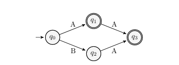
The language L of an FSA A is the set of strings accepted by the FSA, L(A). A string is accepted if there exists a path in A from the starte state q0 to an accepting state. Figure 2.1 gives an example of a simple FSA that encodes strings of lengths one and two over the alphabet A-Z. This work uses the word automaton to reference FSA.

Various types of automata are used to model strings. A majority of research on automata-based string models manipulate unbounded-automata [4,9,18,20–22]. Unbounded-automata are space efficient because they contain cycles, i.e., when a state can have a path to itself. This allows an unbounded-automaton with finite states to represent infinitely many strings. Unbounded-automata do not encode information about length, so there is no inherent mechanism to prevent endless traversal of a cycle, which test case generation requires for better precision. In order to represent strings of finite length, i.e., to create bounded-automata, a sep arate mechanism to enforce bounds is added to the unbounded model. Figure 2.2a
presents a bounded-automaton for string S1, sum of={A-Z}, 0 k 2. This automatonrequires only one state and transition, with the length tracked separately.

In contrast to the bounded-automata, acyclic-automata do not contain cycles, and maintain bounds on length internally. Acyclic-automata are not as space efficient as bounded-automata, as Figure 2.2b shows the acyclic-automaton for string S1 requires three states and two transitions. Since an acyclic-automaton has no cycles and a finite number of states, its language is finite. Another consideration is that applying a string operation to a bounded-automata string model can lead to over-approximation. This is due to the fact that the bounded-automata does not encode length internally [8,16]. Figure 2.3 presents an example from [8] when bounded-automata over-approximates operations. Figure 2.3a shows the unbounded-automaton for strings S1, S2, ={A-Z}, 1 k 2. Then, after concatenate(S1, S2), a new automaton is produced as shown in Figure 2.3b. Since the possible values for S1 and S2 are {A, AA, BA}, the concatenate operation should result in the values {AA, AAA, ABA, BAA, AAAA, AABA, BAAA, BABA}. However, the bounded-automaton in Figure 2.3b accepts the additional values {ABAA, ABBA, BBAA}. This over-approximation is caused by the lack of length information in the bounded-automata. In contrast, the example in Figure 2.4 of acyclic-automata concatenation from [8] shows that a larger acyclic-automaton accepts the correct strings {AA, AAA, ABA, BAA, AAAA, AABA, BAAA, BABA}.
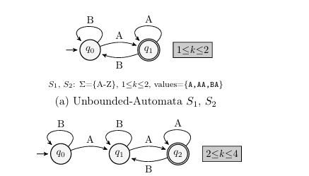

result: ={A-Z}, 2 k 4, values={A,AAA,ABA,BAA,AAAA,AABA,BAAA,BABA,ABAA,ABBA,BBAA}
(b) Unbounded-Automaton Concatenate (S1, S2)
Figure 2.3: Over-Approximation with Unbounded-Automata

S1, S2: ={A-Z}, 1 k 2, values={A,AA,BA}
(a) Acyclic-Automata S1, S2

result: ={A-Z}, 2 k 4, values={AA,AAA,ABA,BAA,AAAA,AABA,BAAA,BABA}
(b) Acyclic-Automata Concatenate (S1, S2)
Figure 2.4: Avoiding Over-Approximation with Acyclic-Automata
Several works of Bultan et al. [18,19] use multi-track automata to model sets of strings. In particular, STRANGER [20] represents symbolic strings as multi-track automata implemented as Multi-terminal Binary Decision Diagrams [6] (MTBDD) using MONA [13]. Other examined works employ fixed-size, ordered, lists of bits called bit-vectors [11, 14, 23] to encode strings, and research indicates bit-vector string models demonstrate performance advantages compared to automata string models [15]. This work focuses on simple, single track automata as a method for representing strings.
2.2 Solvers
Advances in research on string constraints resulted in addtional string constraint solvers supporting diverse analyses. While a comprehensive examination of all available solvers is outside the scope of this thesis, Table 2.1 presents popular string constraint solvers and relevant to this work properties. The Model column describes the type of string model used: automata, bit-vector, or if the solver is axiom-based. The Type column contains the supported constraint types, where mixed indicates that the solver supports a wider range of constraints than the combination of string and integer constraints. The Semantics column contains the language whose string operation semantics the solver implements. The Application column presents the targeted task used in the solver evaluation.
Table 2.1: Popular String Constraint Solvers
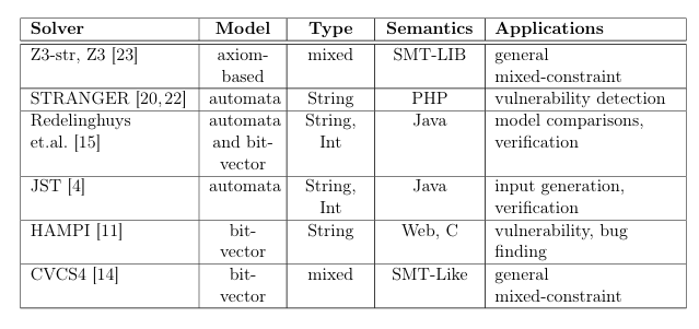

The work presented by Redelinghuys et al. [15] compares automata and bit vector based symbolic string models. While the work focuses on this comparison, it provides insights into the relative merit of the two most widely used types of string models.
The string constraint solver Z3-str [23] implements semantics of the SMT LIB [2] string theory, which might differ from semantics of a particular program ming language. This solver is integrated into the Satisfiability Modulo Theory (SMT) solver Z3. SMT solvers convert a formula in a particular theory into Boolean satisfiability formula that are then passed to a satisfiability (SAT) solver. SMTsolvers handle mixed-constraints by first solving constraints in one theory and then substituting these solutions for variables in constraints for another theory. This process continues until all solvers compute solutions consistent with each other.
CVCS4 [14] is a mixed-constraint SMT solver. However, unlike other SMT solvers, it incorporates techniques for solving string constraints that do not rely upon reduction to satisfiability problems.
HAMPI [11] operates on string constraints that express membership in regular and fixed-size context-free languages. It converts these constraints into bit-vector logic, which is then passed to a solver that supports bit-vector theory. In this regard, HAMPI acts as a pre-processor for other solvers. Designed for vulnerability detection in PHP code, STRANGER [20] performs forward and backward data-flow analysis with automata over control-flow graphs. STRANGER uses a fixed-point solving algorithm that includes widening opera tions in order to ensure convergence. Although similar to the solver presented in this work in most respects, JST [4] computes solutions to both integer and string constraints. It solves mixed con straints in a manner similar to SMT solvers. Both JST [4] and STRANGER [20,22] are most similar to the solver presented in this work, since they are all automata-based solvers.
2.3 Constraint Solving
Now we analyze how these related solvers approach solving string constraints. JST handles mixed constraints of types integer and string. The integer con straints are solved first to obtain concrete integer values that are used in solving string constraints. If no solution can be found for the string constraints, another solution to the integer constraints is generated and the process continues. The solver presented in this work assumes that concrete values are already present in string constraints. While JST uses the same automata library as the solver presented here, dk.brics.automata [4], it uses unbounded instead of acyclic automata models. The authors recognize that over-approximation can occur in the existing string operations, and indicate that some functions require extra
handling [4]. However, it is not apparent that over-approximation is addressed. Bultan et al. provide a body of work on string analysis [1, 3, 18–22], in cluding the string constraint solver STRANGER. STRANGER uses fixed-point calculations to analyze programs using data-flow frameworks. At the start of backwards analysis, an initial work item (automaton) representing the target location (predicate constraint) is placed in a queue. Work items are removed from the queue and pre-string operation automata are computed (similar to inverse string operation in this work). These represent incoming flow values for other work items in the control-flow graph of the program. If the values are different from previously solved incoming flows, then the related work items are updated and placed in the queue. The queue is processed until it is empty, at which point no new incoming flow values are being generated and a fixed-point computation has been achieved. In contrast, the proposed solver analyzes string constraints on a single path in the programs control-flow graph. Details of this proposed framework are presented in the next section. In their other work [19], the authors examine vulnerability analysis using an automata-based solver. Because in that application avoiding over-approximation is not a primary concern, over-approximation is traded for a sound solution. In the context of vulnerability analysis, a sound solution including all vulnerable inputs but with some false-positives is preferable to a solution missing vulnerable inputs but having no false-positives. As a result, the algorithms for computing pre-string operation values in the previous work are not as precise as the ones implemented in this solver.
Relational Constraints

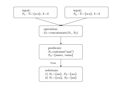
To further improve precision, the solver should maintain relations between certain values. A primary characteristic of this solver is the ability to handle relationships between inputs formed by string operations. Figure 2.5 provides an example of related inputs resulting from the concatenation of symbolic strings S1, S2: ={a-z}, k=2. Solutions for the predicate S3.contains(“aaa”) = true are given, with . Due to the bound on length, (k=2), each input string contributes either one or two characters to the post-predicate values of {aaa , aaa}. Possible values for S1={aa, a} and S2={a , aa}. If input values are chosen for S1 and S2 without regard for the relationship between them, a great number of the resulting combinations do not reach the correct branch.
F. Yu et al. [18] compute solutions for related inputs with the use of memory intensive, computationally complex multi-track automata. This type of automata encodes related values, such as the possible values for the prefix and suffix of a concatenation operation. In contrast, this proposed solver implements an approach of iteratively propagating concrete values for related inputs. The next section presents details of the proposed approach.
SECTION 3
APPROACH
The key elements for successfully implementing the proposed solver are the back ward analysis and inverse string operations algorithms. The general approach to performing the backward analysis is to create a transposed constraint graph (TCG) in which the nodes contain a majority of the required functionality. Essentially the backward analysis traverses the TCG. The basic approach is to compute and propagate incoming and outgoing values at each node, and traverse the TCG with the help of the evaluation stack.
The implementations of inverse string operations depend on the type of the operation. The most straightforward approach is for those inverse operations that return sound and complete results. For inverse operations that return sound but incomplete results, the solver eliminates the incompleteness. Finally, inverse operations that deal with related inputs rely on the framework algorithm for soundness.
The answer to two research questions introduced in Section 1.5 guides the presentation of this section:
RQ1
Can all inverse string operations be accurately modeled? Section 3.2.1
provides formal definitions for the inverse string operations that positively answer this question. To help with answering RQ1, we partitioned it into a series of the following questions:
Does over-approximation occur in an inverse operation and if so then how is it mitigated? Section 3.1.7 presents the over-approximating inverse operations and the solution to handling such over-approximations.
Can existing string operations be used to model inverse operations? Section 3.2.1 provides examples of inverse string operations modeled with existing string oper ations such as insert(int index, String arg) 1 and reverse() 1.
How to define inverse operations that cannot be expressed with existing au tomata operations? Operations such as toLowerCase() 1 cannot be defined in terms of existing string operations. Directly modifying the automata that encodes the string values provides a way to implement these inverse functions. Section 3.1.7 describes such modifications.
RQ2
How to maintain dependencies between string values while solving string constraints for solutions? Section 3.1.8 explains how related data-flow values are determined and propogated in a way that maintains their relationships. The following Section 3.1 details the backward analysis in a presence of un sound, but complete inverse operations. After that Section 3.2 focuses on inverse operations.
3.1 Backward Analysis
3.1.1 Constraint Graph
Before the backward analysis begins, the solver performs the forward analysis on a string constraint graph that encodes string constraints: its nodes are expressions and edges data-flow of string values between them. Figure 3.1 presents an example constraint graph, where nodes are string inputs (node 5), operations (nodes 10 and 17), predicates (node 32) and concrete strings (node 30).

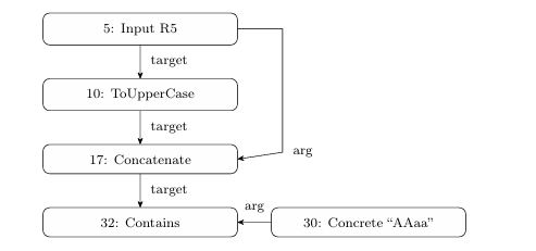
Directed labeled edges specify type of data uses, which can be either target or argument for the destination node. In object-oriented terms, the target is the string object (automaton) on which the instance method (string operation) is called. Nodes in the constraint graph can have multiple incoming and outgoing edges. Each outgoing edge indicates a use of the node’s outgoing value. Each node contains a numerical identifier (node ID) indicating an order for evaluating nodes during forward analysis. The forward analysis traverses the constraint graph in total-order on node ID until it determines the possible string values at a predicate node and evaluates it to true or false.
3.1.2 Transposed Constraint Graph

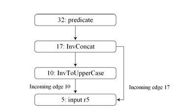
Backward analysis starts after forward analysis completes the evaluation of a predicate node. The framework builds a TCG, consisting of inverse constraint nodes, while reversing (or transposing) edge directions from the constraint graph. In a TCG, a node may have multiple incoming edges representing multiple uses of a value. Figure 3.2 shows the TCG of the constraint graph in Figure 3.1. Note that “input r5” has multiple incoming edges since it is the target of the toUpperCase() string operation as well as the argument to the concat() string operation in the constraint graph. In order to find a solution for input r5, the values of all the incoming edges must have a common element. Each inverse node contains a solution set that keeps a set of solutions from each incoming edge. A solution set is said to be consistent when the intersection of all its elements is not empty. Figure 3.3 shows a diagram of an inverse constraint node and its solution set.

3.1.3 Graph Traversal
Backward analysis starts at the post-predicate values and propagates their results toward the input nodes by performing a depth-first traversal of the TCG. The solver maintains a stack of nodes to be evaluated, and initializes it with the pred icate. Here, the evaluation stack is an abstract concept and can be implemented as either an actual stack or as a series of function calls in which each node calls the evaluate(inputNode, sourceIndex) function on the next inverse constraint node in the TCG. The algorithms presented here use the latter.
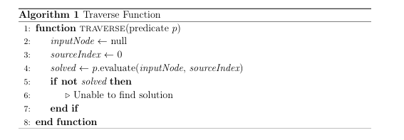
Algorithm
Algorithm 1 depicts a pseudocode for the traversal algorithm in which each node calls the evaluate(inputNode, sourceIndex) method on the next (target) node in the TCG. Below are the assumptions that Algorithm 1 relies on:
• Each node in the TCG has references to its children and parents.
• Each incoming edge represents a use of the node output in the original
constraint graph.
• Each node has access to the results of the forward analysis.
The algorithm takes as input a predicate node p of the TCG. Each node’s evalu ate method takes two arguments: a reference to the calling node (the predecessor of the called node) and an integer that indicates which output to take from the calling node. Some nodes, such as those that handle related values, have multiple outputs. In the case of a predicate node, there is no predecessor and the input will be the output of the next node. The algorithm sets inputNode and sourceIndex accord ingly and begins the traversal by calling evaluate(inputNode, sourceIndex) on the predicate node. If the returned value is false, then the solver has failed to find a solution, or the predicate was UNSAT.

3.1.4 Fallback Sequence
A fallback sequence begins when the evaluate function of a node returns false. Once initiated, a fallback sequence continues until:
A node has more values to propagate- Since unsound nodes propagate a subset of incoming values, it is possible that other unexplored values could lead to a consistent solution.
A predicate is reached- This serves as a check for defects. If a predicate has satisfiable assignments after the forward analysis, then there are corresponding inputs for those assignments. If the evaluate(inputNode, sourceIndex) call in a predicate returns false, then the solver has failed to find those inputs.
3.1.5 Node Evaluation
Each node calls the evaluate(inputNode, sourceIndex) functon on the next node in the TCG. The function is different for each node type. The node types are:
• Predicate Node
• Input Node
• Inverse String Operation Node- Operation that is Sound and Complete
• Inverse String Operation Node- Operation that Over-Approximates (Sound
but Incomplete)
• Inverse String Operation Node- Relational String Operation (Unsound but
Complete)
Predicate node evaluation propagates the post-predicate values and calls evaluate(inputNode, sourceIndex) to the next node. Since all arguments to a predicate are concrete, there is only one node following a predicate, i.e., the “target”. Algorithm 2 presents the pseudocode for evaluating predicate nodes. The forward results of the next node are retrieved on line 2. If the results contain values, they are placed in the output set on line 4. The output set contains one or more sets of values for subsequent nodes to use as input. The algorithm then calls evaluate(inputNode, sourceIndex) on the next node in the TCG and returns the boolean result.


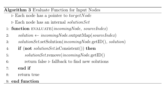
Since a node may have more than one parent, a construct is needed to keep all of the inputs from these calling nodes and determine if they are consistent. Each node has a solution set for this purpose, and it is said to be consistent if the intersection of all inputs in the set is not empty. The evaluate(inputNode, sourceIndex) function for input nodes demonstrates use of the solution set. Algorithm 3 presents the pseudocode for evaluating input nodes. The solution (input) from the calling node is retrieved on line 2. It is placed into a solution set on line 3. The solution set is checked for consistency on line 4 and if the solution set is not consistent the solution is removed on line 5 and a fallback is initiated on line 6 by returning false. If the solution set is consistent, the function returns true, as an input node has no child nodes (i.e., no next node to evaluate).

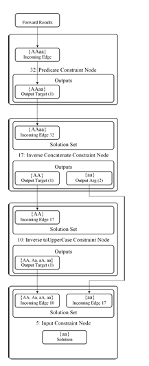
The algorithm starts with a predicate, 32, which has the value satisfying it “AAaa”. String values generated by each inverse operation are shown in each node. As solutions are added to the solution set of r5, they are intersected with all existing solutions in the solution set. If the intersection does not contain any values, a fallback sequence is started in an attempt to find new solutions. A solution is found for r5 once all incoming edges have been evaluated and the solution set is consistent. All incoming edges for all input nodes are considered evaluated once the series of evaluate calls completes. In this case, the solution is the intersection of incoming edge 10 and 17, which is “aa”. Using “aa” as the value input r5 in the constraint graph in Figure 3.1 shows that the true branch is taken, and the solution is correct. The algorithm relies on correct implementation of inverse operations, which
are detailed in the next section.

3.1.6 Sound and Complete Operations
String operations can be either injective or non-injective. Non-injective operations map more than one input to the same output. Injective operations map a single input to an output. In situations where the solver has sufficient information about an injective string operation, a sound and complete inverse result can be computed. Algorithm 4 presents the pseudocode for the evaluate(inputNode, sourceIndex) for sound and complete nodes. The input is retrieved from the calling node on line 2. The inverse operation is applied on line 3. Lines 4-8 add the results to the solution set and check for consistency, returning false if the solution set is not consistent. If the solution set is consistent, lines 9-10 add the solution to the output set and call evaluate(inputNode, sourceIndex) on the next node. 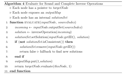

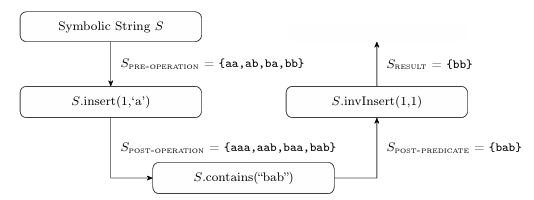
To illustrate the algorithm, consider Figure 3.5 that shows the flow of a sym bolic string through a forward string operation, predicate, and backward anal ysis with a sound and complete inverse string operation. In this example the string operation is insert(int offset, char c): S.insert(1,‘a’). The predicate is S.contains(“bab”). String S is defined with parameters k=2 and ={a,b}. The edges are labeled with the values for S. The inverse string operation is S.invInsert(1,1), which deletes a single character at index one. The result is the single value “bb”, which is both sound and complete. In this case the solver has sufficient information (length and position) to remove the inserted character sequence to compute an accurate result. In this context, the insert operation is injective, as there is only one possible input value, “bb”, that results in the output value “bab”.

3.1.7 Handling Over-Approximation
A non-injective string operation results in unavoidable over-approximation in its inverse string operation. A common approach for eliminating over-approximation is to intersect the over-approximated result with the results of the forward analy sis [21]. This step removes the spurious strings introduced by the over-approximating
inverse. The evaluate(inputNode, sourceIndex) function for a node with an over approximating inverse string operation performs the intersection required to elim inate the over-approximation. Algorithm 5 presents the pseudocode for such a function, with the intersection occurring on line 4.
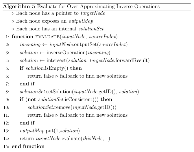

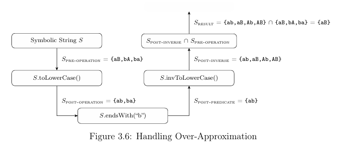
Figure 3.6 gives an example of the non-injective string function toLowerCase() and the subsequent over-approximation in invToLowerCase(). Given a string S,
={a, b, A, B}, k=2, whichhastheinitial values {aB, bA, ba}, the toLowerCase() function produces Spost-operation = {ab, ba}. Application of the predicate pro duces Spost-predicate = {ab}, which is input to the invToLowerCase() operation. However, the lower case string “ab” is the result of calling toLowerCase() on any of the strings {ab, aB, Ab, AB}, with only one of the four present in Spre-operation. Intersecting Spre-operation with Spost-inverse eliminates the additional strings intro duced by invToLowerCase().

3.1.8 Maintaining Related Values
Unsound results are returned when an inverse string operation needs to maintain the relationship of outgoing strings. However, single-track automata models can not maintain such relations. Each string model represents one string, with no intrinsic way to specify a relationship with a string from another node. Previous work examines methods of handling string relations using complex, multi-track automata that are memory and computationally expensive [18,19]. The approach taken here focuses on completeness, and it propagates singleton values as matched pairs for related concrete strings. To ensure soundness, the framework produces all matched pairs through iteration. The related value node evaluate(inputNode, sourceIndex) function is pre sented in Algorithm 6. The function maintains the list of related values returned by the inverse string operation, and either returns values from this list if available, or uses the inverse string operation to generate more values from remaining input.
The input is retrieved from the calling node on line 2. The alogrithm selects concrete values from these inputs, and the while loop initiated on line 3 continues until all inputs are exhuasted or solutions are found. Line 4-5 remove a concrete value from the inputs. Lines 6-7 retrieve string models from the target and
argument nodes. Line 8 calls the inverse operation that returns a set of tuples, each tuple containing a matched pair of concrete values that satisfy both the target and argument nodes. The while loop initiated on line 9 continues until all of these tuples have been propagated or a solution is found. Line 10 removes a single tuple
from the set. It is split into two singleton string models on lines 11-12. The singleton string models are intersected with the forward results on lines 13-14. The singleton string models are placed in the output set on lines 15-16. The evaluate(inputNode, sourceIndex) function for both the target and argument nodes is called on line 17. If both of these calls return true, then the algorithm returns true. If no solution is found and all available values have been explored, the algorithm returns false.
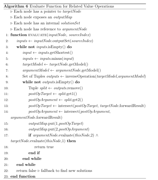

Figure 3.7 presents the flow of related symbolic strings through a concatena tion operation, where input strings S1, S2 are defined with parameters ={a,b}, 1 k 2. The post-predicate values for S3 are displayed below the invConcat() node. In this example, the string value “aaa” (underlined in the figure) is selected
as input to the invConcat() operation. The invConcat() operation returns a list of valid prefix / suffix pairs for further computations. In this case it returns tuples (a, aa) and (aa, a). The first singleton values propagated are S1 = “a”, S2 = “aa”. If a fallback occurs or multiple solutions are needed, then the next
evaluation returns S1 = “aa”, S2 = “a”. After that, another singleton is removed from the set of incoming values and the process continues. If no further pairs are available and there are no further incoming values available, a fallback sequence is initiated. It is important to note that the invConcat() exhaustively returns all of the prefix / suffix pairs, which makes this operation sound and complete.
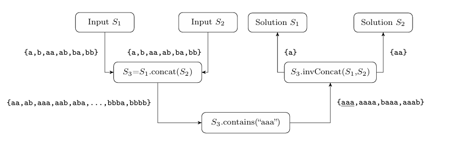

Figure 3.7: Handling Related Inputs
This approach addresses the goals of prioritizing a complete solution over a sound solution in a single iteration, while maintaining relationships between string inputs. Note that the term unsound result when applied to an inverse string operation using this approach means it has not yet returned all of the values in a sound result, but does not indicate that it cannot produce a sound result if it is allowed to exhaust the incoming values.
3.1.9 Termination
The algorithm terminates since the TCG is acyclic, and each node has a finite
number of values that it can propagate backwards. It finds a solution because it
propagates all feasible predicate strings backwards to each input, and one of those
strings must lead to a solution.
3.1.10 Complexity
The nodes of the TCG can be partitioned into two groups: source and sink nodes, and inverse operation (inner) nodes. Source and sink nodes are predicates, inputs, and constants. These three node types simply propagate values, with the input nodes taking the additional step of checking the solution set for consistency. Here we define aninput size as the number of values the symbolic string inputs represent. Since the input size does not affect these nodes, they compute in constant time. Note that the number of values a symbolic string input represents is determined by the alphabet and the length of input strings. Inverse operation nodes can further be categorized into two types: Those that return a full solution (sound) and those that do not (unsound). The complexity of inverse operations of sound nodes depend on the input size and has growth linear with the automata size. The complexity of inverse operations for the nodes that compute unsound results has non-linear growth with the input size. A worst-case scenario, therefore, is a constraint containing multiple unsound operations over related variables such as s1.concat(s1) 1. Consider unsound nodes in the TCG. We define d as the size of their inputs, set in this case the number of string values output by the previous node. Note that d depends on the length and alphabet size of the symbolic string inputs (see Section 5.3 for more details). We define p as the maximum number of matching tuples of values for each d input value that such node can produce. In a worst case scenario all of these pairs need to be propagated to the descendants of the node. We define m as the number of inverse operations in the TCG. Then the resulting recurrence relationship is f(m) = d p f(m 1). This reduces to f(m) = dm pm, which is the worst case number of traversals of the TCG.
3.1.11 Limitations
The algorithm is limited in the handling of multiple predicates. Although a constraint graph may have multiple predicates present, the algorithm processes one predicate at a time, without consideration for the presence of others. In practical terms, the algorithm cannot reliably process related predicates such as embedded “If” statements. It will solve each independently and cannot backtrack to previously solved predicates. Extension of the algorithm to multiple related predicates is left for future work.
3.2 Inverse String Operations
Nodes in the TCG ally with inverse string operations for the backward analysis. The following list itemizes the properties of an inverse string operation:
• All operations must return complete results.
• Some operations return sound and complete results on the first evaluation.
• When relationships between strings must be maintained, an operation re turns an unsound result containing a set of singleton pairs.
• Operations that return unsound results can be repeatedly queried until all possible results are returned.
• When over-approximation occurs, inverse results are intersected with pre string operation values to obtain a complete result.
3.2.1 Formal Definitions and Algorithms
The formal definitions are based on the following assumptions. First, each inverse operation takes as input an acyclic-automata A encoding all of the possible strings from the previous inverse operation. However, the inverse concatenation operation only considers singletons to compute the prefix and suffix inverses. Second, all of the string operations modeled in the forward analysis such as delete and insert are available, as well as standard automata operations such as union and intersection. Third, all integers used in arguments of string operations such as substring have concrete values.
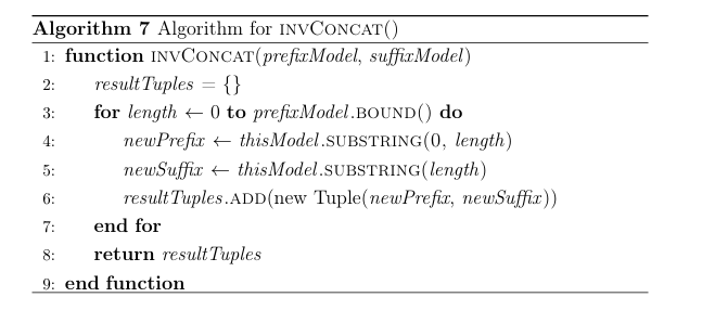
Inverse String Operation t.concat(String arg) 1:
From the input automata, a single string s is removed and encoded in A. Then the inverse is defined as: (t arg) i
[0 s] t = Asubstring(0 i) arg = Asubstring(i) The inverse of concat operates on a single string s and splits it into all possible prefix and suffix combinations. This inverse produces a set of (t arg) tuples for each possible i split. The pseudocode for inverse concatenate is presented in Algorithm 7. At line 3 it iterates over the length of the prefix. Each iteration builds a prefix / suffix tuple on lines 4-5. A new tuple is created and added to the result set on line 6. A set of tuples containing all feasible prefix / suffix pairs is returned on line 8. The evaluate(inputNode, sourceIndex) removes infeasible tuples from the result tuples.

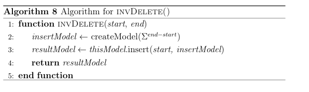
Inverse String Operation t.delete(int start, int end) 1:
Let Asubstr have L(Asubstr) = end start, that is all strings of length (end- start). The inverse is defined as: Ainsert(Asubstr start) All possible strings of length (end start) are inserted into A. The pseudocode for inverse delete is presented in Algorithm 8. A new symbolic string accepting all strings of the length of the deleted portion is created on line 2. The new symbolic string is inserted into the target automaton on line 3. Subsequent intersection with forward results occurs in the calling evaluate(inputNode, sourceIndex) function.

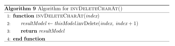
Inverse String Operation t.deleteCharAt(int index) 1:
The inverse is defined in terms of the t.delete(int start, int end) 1.
The inverse is:
t.delete(int index, int index + 1) 1
The pseudocode for inverse deleteCharAt is presented in Algorithm 9. Line
2 assigns the value of a call to the invDelete function with arguments that evaluate to a string of length one.

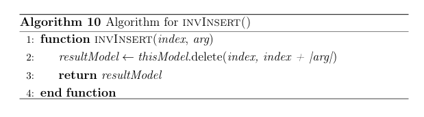
Inverse String Operation t.insert(int index, String arg) 1:
Let A be the target string model. Let m be arg, where arg is a concrete string, then the inverse is defined as:
A.delete(index, m)
This inverse operation deletes a substring of length m at the specified location. The algorithm for inverse insert is presented in Algorithm 10.
Line 2 assigns the value returned by a delete invocation, which removes the inserted portion from the target symbolic string.

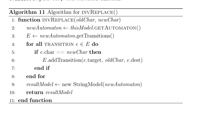
Inverse newChar) 1: String
newChar) 1:
t.replace(char oldChar, char Let A = (Q Eq0F) be the incoming automaton. Given the
values of oldChar and newChar, define a new set of transitions Et = E (poldChar q) (pnewChar q) E . The inverse creates a new automaton with a new set of transitions Et, that is the automaton for the target becomes:
(Q Et q0F)
This inverse operation adds additional transitions with oldChar labels to A between states that already have newChar as labels. The pseudocode for inverse replace is presented in Algorithm 11. Line 2 extracts the underlying automaton from the symbolic string, since the function directly modifies it. The sets of transitions are initialized on line
3. Lines 4-8 iterate over all of the incoming automata transitions, adding a new oldChar transition to the new transition set for every newChar transition. Line 9 creates a new automaton and string model.
Subsequent intersection with forward results occurs in the calling evaluate(inputNode, sourceIndex) function.

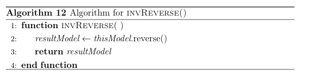
Inverse String Operation t.reverse() 1:
Let A be the target string model. The inverse is defined as:
Areverse()
The reverse operation is the inverse of itself and has no over approximation. The pseudocode for inverse reverse is presented in Al-gorithm 12. The algorithm simply invokes reverse on the string model on line 2

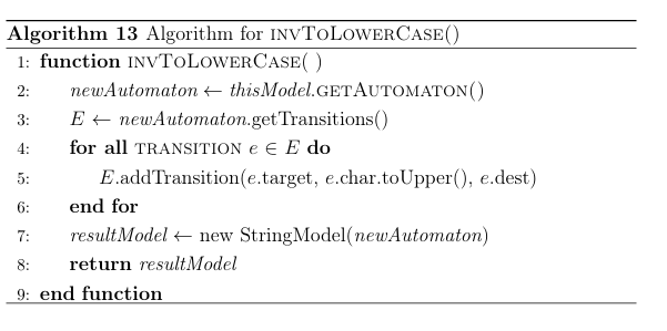
Inverse String Operation t.toLowerCase() 1:
Let A = (Q Eq0F) be the incoming target automaton. We define a new set of transitions Et = E (pupperCase(char) q) (pcharq)
E . The inverse operation creates a new automaton with the new set of transitions Et. The inverse is defined as the new automaton: (Q Et q0F)
The inverse adds a transition with an upper case character between states that have transitions on a corresponding lower case character. The algorithm for inverse toLowerCase is presented in Algorithm 13. A reference to the underlying automaton is created on line 2. Lines 4-6 iterate over the transitions and characters. Line 5 adds an upper case transition for every character. Subsequent intersection with forward results occurs in the calling evaluate(inputNode, sourceIndex) function.

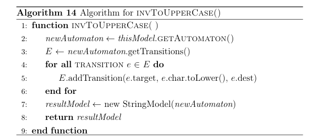
Inverse String Operation t.to Upper Case() 1:
Let A = (Q Eq0F) be the incoming target automaton. We define a new set of transitions Et = E
(p lowerCase(char) q) (pcharq)
E . The inverse operation creates a new automaton with the new set of transitions Et. The inverse is defined as the new automaton: (Q Et q0F)
The inverse adds a transition with a lower case character between states that have transitions on a corresponding upper case character. The algorithm for inverse to Upper Case is presented in Algorithm 14. A reference to the underlying automaton is created on line 2. Lines 4-6 iterate over the transitions and characters. Line 5 adds a lower case transition for every character. Subsequent intersection with forward results occurs in the calling evaluate(input Node, source Index) function.

Inverse String Operation t.substring(int start, int end) 1:
Let A be the incoming target automata. Define m as the maximum length of string in the forward results AF
0 and an automaton Aprefix such
that L(Aprefix) = start. Define automaton Asuffix such that L(Asuffix) =
m end. Then the inverse is defined as follows:
Aprefix concat(A) concat (Asuffix)
The pseudocode for inverse substring(start, end) is presented in Algo rithm 15. It creates a prefix of known length start and a suffix of length m endaccepting all strings to the given length. It then concatenates the Aprefix, A, and Asuffix. Line 2 creates a string model that accepts strings up to the length of the removed prefix. Line 3 creates a suffix model that is at least as long as the removed suffix. Line 4 concatenates the prefix, target and suffix together. Subsequent intersection with forward results occurs in the calling evaluate(inputNode, sourceIndex) function. 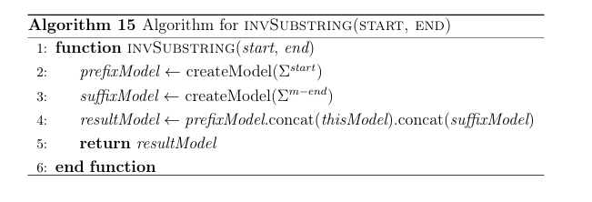

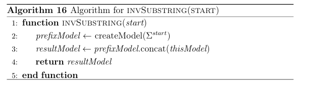
Inverse String Operation t.substring(int start) 1:
Let A be the incoming target automata. Define automata Aprefix such that L(Aprefix) = start. The inverse is defined as:
Aprefix concat(A)
The pseudocode for inverse substring(start) is presented in Algorithm 16. It creates a prefix of known length start accepting all strings to the given length. It then concatenates the Aprefix and A. A prefix model is created that accepts all strings up to the length of the removed prefix on line 2. Line 3 concatenates the prefix and target. Subsequent intersection with forward results occurs in the calling evaluate(inputNode, sourceIndex) function.

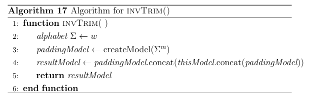
Inverse String Operation t.trim() 1:
Let A be the incoming target automata. Define w as the whitespace character, and m as the maximum length of string in the forward results AF 0. Define Apadding such that L(Apadding) = wm. Then the inverse is
defined as:
Apadding.concat(A.concat(Apadding))
The pseudocode for inverse trim is presented in Algorithm 17. The inverse operation pads the strings encoded in A with the whitespace character such that all strings are at least as long as the longest string in AF 0. A string model as long as the maximum string length is created on line 3 that accepts all strings comprised of the whitespace character. The prefix, target and suffix are concatenated on line 4. Subsequent intersection with forward results occurs in the calling evaluate(inputNode, sourceIndex) function.

SECTION 4
IMPLEMENTATION
The solver is part of a larger input generation framework shown in Figure 4.1. The solver has been completed, extending the code from previous research comparing the performance of string solvers [10]1 and the suitability of automata for modeling symbolic strings [16]2. These in turn are largely based on Java String Analyzer (JSA) and the dk.brics automaton library [4]3. The input generation framework is part of the public repository at
https://github.com/BoiseState/string-constraint-counting.
The framework consists of the following components, illustrated in Figure 4.1: Input Generator- This is the main entry point for the system. It instantiates the reporter, parser, and solver. It instantiates the reporter run() function, which in turn uses the parser and solver to generate inputs through backward analysis. Parser- Parses input graphs encoding into internal data structure. Solver- Contains forward and backward analysis logic as well as the symbolic string table.
1https://github.com/BoiseState/string-constraint-solvers
2https://github.com/BoiseState/string-constraint-counting
3http://www.brics.dk/JSA/, https://www.brics.dk/automaton/

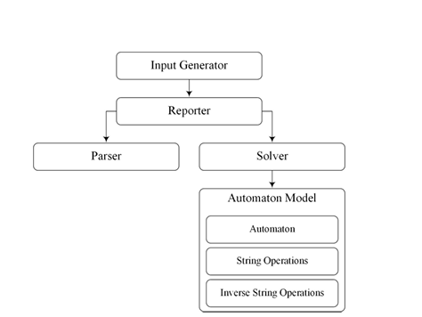
Reporter- Bridges the parser and solver components, and provides output from the system.
Automata Model- Contains the acyclic automata and implementations of string operations and their inverse.
Table 4.1 presents Software metrics of the initial (string-constraint-counting) and current (inverse-testing) codebases. The implementation adheres to object oriented design principles, with proper type hierarchy represented by interfaces, abstract classes, and concrete classes. This results in a larger increase in the number of classes and interfaces in comparison to lines of code.
Table 4.1: Metrics for Initial and Current Codebase
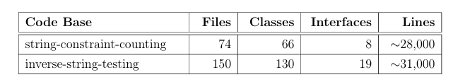

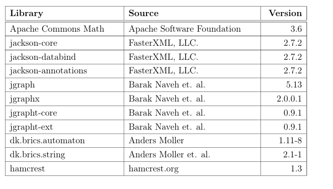
Table 4.2 contains the external dependencies required to build the input gen-eration system.
Table 4.2: Major Dependencies

4.1 Inverse String Operation Classes
Interfaces and base abstract classes specify the inverse string operations and meth ods necessary to perform the backward analysis. The acyclic-automata model is extended with the inverse string operations shown in Table 4.3. String operations may have multiple inverse string operations, depending on the argument types passed to the string operation, i.e., whether the argument is concrete or symbolic. The Sound column indicates whether the inverse operation returns a sound result on the first evaluation. The Over column indicates whether the inverse operation over-approximates.
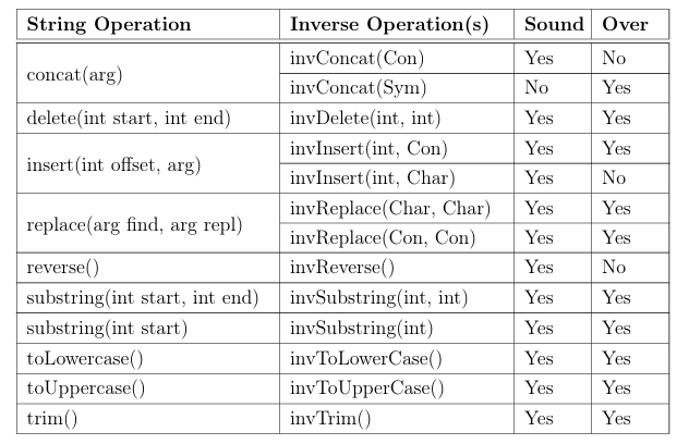

4.2 Solver
Interfaces and base abstract classes include the methods for supporting backward analysis and performing inverse string operations. The solver class has been extended to support the inverse string operations implemented in the acyclic automata string model.
The solver takes as input a constraint graph stored in a JSON format. The JSON file encodes the edge and vertices information along with the alphabet definition. Input length can be optionally encoded in the file or specified through command line arguments.
Benchmark constraint graphs are collected in previous work [10,16] by instru menting real-world Java programs.
4.3 Integration with Symbolic Pathfinder
The input generation system is loosely integrated with Symbolic Pathfinder (SPF). Currently SPF does not support many of the non-injective functions that the solver can currently perform. For those benchmarks that include only those functions SPF supports, a semi-automated workflow has been developed. First, SPF analyzes the Java program and produces a path condition, which is parsed into a JSON file for input into the system. Figure 4.2 shows the workflow for this process. Figure 4.3 shows an excerpt from a Java program used for correctness testing and the resulting path condition from SPF. Figure 4.4 shows the resulting constraint graph.
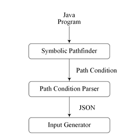

Figure 4.2: Symbolic Pathfinder Data Flow
1 public class BSU_SCS_Inverse_case_6 {
2 …
3 // method under test
4 public static void mut(String r5) {
5 if (r5.substring(4, 7).equals(“two”)) {
6 pathTaken = path != 0 ? 1 : 0;
7 return;
8 } else {
9 pathTaken = path != 0 ? 2 : 0;
10 return;
11 }
12 }
13 }
14
(a)Methodwithstringinput
(r5-1-SYMSTRING.substr(4,7)equals CONST-two)
(b)PathConditionsfromSPF
Figure4.3:ExampleSPFInputandOutput

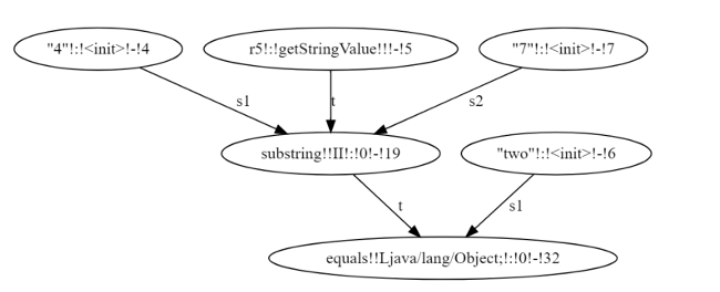
SECTION 5
EVALUATION
This section provides details on the correctness verification as well as the answer to research question RQ3: Is the solution practical and effective?
5.1 Correctness
Fifteen synthetic test cases are used to verify correctness, developed specifically for this solver. They are implemented as Java programs where string inputs determine execution paths, taking as input concrete string values and expected execution paths for them. Figure 5.7 presents the test flow diagram from a Java program through verification results. The Java test case program is used as the input into SPF, with method Under Test() specified as the target method for analysis. SPF generates a path condition which is then parsed into a JSON file containing the constraint graph. This in turn is used as input into the Input Generation framework which uses the solver to generate a solution for each parameter of method Under Test(). Correctness is verified by executing the Java test case program with the solution values and observing the results. The test cases are designed such that they indicate success or failure based on the expected and actual path taken with the computed input values. Some of these test programs incorporate non-injective an unsound operations. Thus, Figure 5.1 presents a test case incorporating non-injective and un sound operations on line 26. This code corresponds to the constraint graph in Figure 5.2. Other test cases take multiple inputs (Figures 5.5 and 5.6)and have multiple out going edges from a node(Figures 5.3 and 5.4) in their constraint graphs. These test cases compose the correctness benchmark.
1 public class BSU_SCS_Inverse_case_1 {
2 static int path = 0;
3 static int path Taken = 0;
4 static String r5;
5 static boolean test = false;
6
7 public static void main(String[] args) {
8 if (args.length == 2) {
9 path = Integer. parse Int(args[0]);
10 r5 = args[1];
11 test = true;
12 System. out. print ln(“\nTEST: Args … ” + r5 + “\nTEST: Path … ” + path);
13 } else {
14 r 5 = “A”; }
15
16 method Under Test(r5);
17
18 if (test) {
19 if (path- path Taken == 0) {
20 System. out. print l n(“TEST: SUCCESS”);
21 } else {
22 System. out .print l n(“TEST: FAILURE”);
23 } } }
24
25 public static void method Under Test(String r5) {
26 if (r 5. to Lower Case().con cat(“AB”).contains(“a A”)) {
27 path Taken = path != 0 ? 1 : 0;
28 return;
29 } else {
30 pathTaken = path != 0 ? 2 : 0;
31 return;
32 } } }
33
Figure 5.1:Non-Injective and Unsound Operations Test Case Code

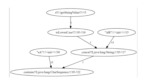
1 public class BSU_SCS_Inverse_case_1a {
2 static int path = 0;
3 static int pathTaken = 0;
4 static String r5;
5 static boolean test = false;
6
7 public static void main(String[] args) {
8 if (args.length == 2) {
9 path = Integer.parseInt(args[0]);
10 r5 = args[1];
11 test = true;
12 System.out.println(“\nTEST: Args … ” + r5 + “\nTEST: Path … ” + path);
13 } else {
14 r5 = “A”; }
15
16 method UnderTest(r5);
17
18 if (test) {
19 if (path- path Taken == 0) {
20 System. out. println(“TEST: SUCCESS”);
21 } else {
22 System.out. println(“TEST: FAILURE”);
23 } } }
24
25 public static void method Under Test(String r5) {
26 if (r5. contains(“aA”)) {
27 if (r5.contains(“AA”)) {
28 pathTaken = path != 0 ? 1 : 0;
29 }
30 return;
31 } else {
32 path Taken = path != 0 ? 2 : 0;
33 return;
34 } } }
35
Figure 5.3: Multiple Outgoing Edges Test Case Code

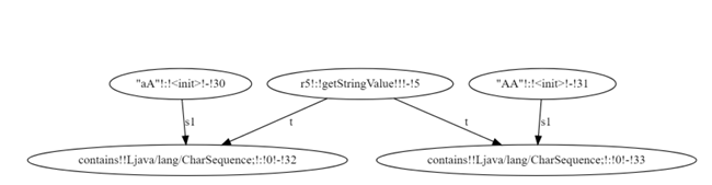
1 public class BSU_SCS_Inverse_case_2 b {
2 static int path = 0;
3 static int path Taken = 0;
4 static String r 5,r 6;
5 static boolean test = false;
6
7 public static void main(String[] args) {
8 if (args.length == 3) {
9 path = Integer. parse Int(args[0]);
10 r5 = args[1];
11 r6 = args[2];
12 test = true;
13 System. out. print ln(“\nTEST: Args…r 5: “+r5+” r6: “+r6+”\n TEST: Path…”+path);
14 } else {
15 r5 = “one”;
16 r6 = “two”; }
17
18 method Under Test(r5, r6);
19
20 if (test) {
21 if (path- path Taken == 0) {
22 System. out. print ln(“TEST: SUCCESS”);
23 } else {
24 System. out. print ln(“TEST: FAILURE”);
25 } } }
26
27 public static void method Under Test(String r 5, String r 6) {
28 if (r5. con cat(r6).contains(“one two”)) {
29 path Taken = path != 0 ? 1 : 0;
30 return;
31 } else {
32 path Taken = path != 0 ? 2 : 0;
33 return;
34 } } }
35
Figure 5.5: Multiple Inputs Test Case Code
The constraint graph file contains the size and description oft he alphabet,and theboundonlengthsofsymbolicstringinputsinadditiontotheconstraintgraph.
In order to achieve reason able run time son the correct ness benchmark,bound sand

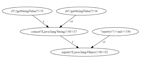

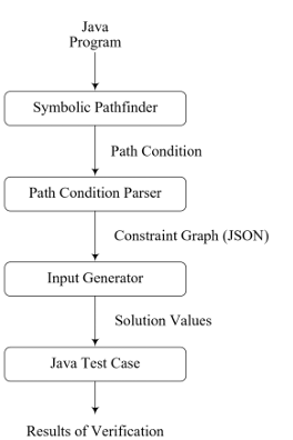
alphabets are set to small values such that testing completes quickly. Alphabets of (A-C, a-c) are used unless additional characters are needed (test cases 2b and 6). The testing iterates over length bounds due to unsoundness of the approach. At each iteration the length bound is incremented, starting with length k = 1 and doubling in length until k = 16.
Test case properties are presented in Table 5.1.
Table 5.1: Test Case Properties
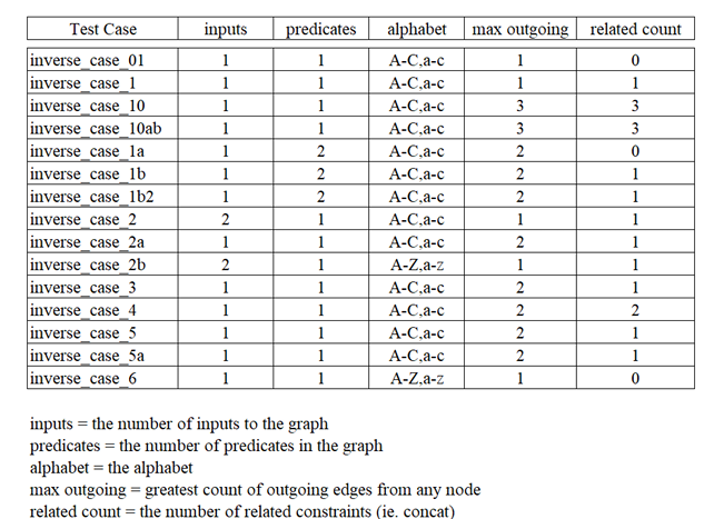

5.1.1 Correctness Results
The correctness experiment is performed on an Intel(R) Xeon(R) CPU E5-2407 v2 @ 2.40GHz based system with 24GB of memory, running Fedora Linux version 33-1.2. The JVM used is OpenJDK version 11, with the target compatibility set to version 1.8. Each benchmark is executed three times with the average performance being reported. Table 5.2 presents performance timing and solution results of the correctness benchmark. The values reported in the input length columns is the time in milliseconds(ms) for the solver to compute a solution at the given length. In those cases where the solver cannot find a solution (NS) it was verified manually that there were no possible solutions due to the given length being too restrictive. Timeouts of greater than 120 minutes are indicated with TO. Only the backward analysis time is presented in the table, however, the timeout calculation includes forward analysis time. The solutions column contains the computed solution to the input(s), and in cases where there is more than one solution only one chosen for an example. Note that once a solution is found at a given length, longer lengths continue to produce solutions unless a time out occurs, which serves as another measure of correctness of the implementation.
Table 5.2: Correctness Results
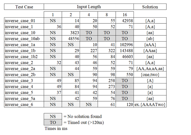

This testing process brought to light multiple faults in the code, but no fund a- mental errors in either the solvers algorithms or the logic of the inverse operations.
All solutions generated for the test cases successfully reach the expected locations when used as inputs to the Java benchmark programs.
To note, all runtime measurements increase as the length bound increases. This is an expected behavior, but some real-world program benchmarks presented in the next section exhibit a different trend.
Test cases 10 and 10ab demonstrate expected inefficiencies of the solver with certain constraints. In particular, these test cases have multiple concat(String arg) 1 constraints with data dependencies. In general, the performance bottleneck exists when establishing consistency between data dependent nodes. In the case of concatenation, the solver propagates partial results of inverse operations to maintain the relationship between the prefix and suffix pair. This can lead to many iterations of prefix / suffix choices and their propagation until satisfiable pairs are found. As length increases, more prefix / suffix pairs are available for iterations, causing an increase in runtime. Both test cases are only able to produce solutions at k = 2 before timing out. Figures 5.8 and 5.9 present the test code and constraint graph for test case 10 ab.
Reproducing Correctness Results
In order to aid in the reproduction of these results, a Docker file is available at
https://github.com/marlinroberts21/string-input-docker. Utilizing this
file, a user can build an image of a linux system housing the test input generation framework and correctness benchmarks.
1 public class BSU_SCS_Inverse_case_10 ab {
2 static int path = 0;
3 static int path Taken = 0;
4 static String r5;
5 static boolean test = false;
6
7 public static void main(String[] args) {
8 if (args.length == 2) {
9 path = Integer.parse Int(args[0]);
10 r5 = args[1];
11 test = true;
12 System.out. println(“\nTEST: Args … ” + r5 + “\n TEST: Path … ” + path);
13 } else {
14 r5 = “ab”; }
15
16 methodUnderTest(r5);
17
18 if (test) {
19 if (path- pathTaken == 0) {
20 System.out. print ln(“TEST: SUCCESS”);
21 } else {
22 System. out. print ln(“TEST: FAILURE”);
23 } } }
24
25 public static void method Under Test(String r 5) {
26 String s1 = r5.to Upper Case();
27 if (r 5. con cat(s1).concat(s1.concat(r5)).contains(“ab”)) {
28 path Taken = path != 0 ? 1 : 0;
29 return;
30 } else {
31 path Taken = path != 0 ? 2 : 0;
32 return;
33 } } }
34
Figure 5.8: Related Unsound Operations Test Code

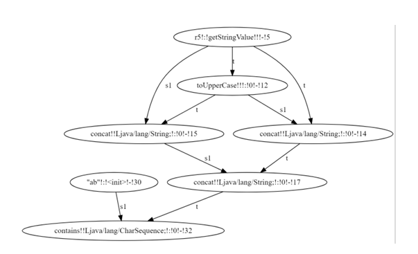
5.2 Practicality
In order to answer the research question Is the solution practical and effective?, definitions of both practical and effective are needed. Practical means that the solver can be used in practice, in contexts of real-world scenarios, that include conditions and inputs. Effective means that the solver finds solutions for the inputs in those contexts.
To demonstrate practicality, it is necessary to have a set of inputs representing actual programs that incorporate common constructs and patterns found in Java programs. Previous work [10,16] obtained such a set of benchmarks from real-world Java programs and encoded them in constraint graphs, discussed previously. The benchmarks consist of a series of constraint graphs for three different Java pro grams, with each representing dynamic execution paths of programs with different concrete inputs. Table 5.3 presents the number of nodes, operations, predicates and inputs of each benchmark.
Table 5.3: Benchmark Properties
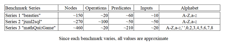

The solver is effective in that it finds solutions for all of the real-world bench marks. Since the programs contain string operations which SPF does not support, it is not possible to incorporate them into the testing framework.
5.2.1 Results
Each benchmark series is executed in the same environment as the correctness benchmark. Similarly, each benchmark is executed three times and the average analysis time is reported.
Series One This series exhibited be havior unlike the correctness benchmarks in that approximately half of the benchmarks had a minimum runtime at length k = 16. Table 5.4 presents the runtimes as a ratio (Run time Minimum Runtime).
The minimum runtime for each benchmark is shaded. Figure 5.10 presents a box
plot of the ratio data from Table 5.4.
Series Two The series two execution times are presented in Table 5.5. This series does not have solutions at any length less than k = 16. This is due to the fact that the predicate arguments in this series can be length k = 11. For instance, in put contains( description ) cannot have a solution for input at any k11. The two outliers identified in the box plot in Figure 5.11 have significantly fewer nodes than the other benchmarks in the same series. This led to significantly lower run times for both benchmarks.
Series Three Similar to series two, this series did not generate solutions until reaching a certain length, k = 8. At k = 16 all but two of the benchmarks reached the timeout of 120 minutes. The two outliers identified in the box plot in Figure 5.12 have significantly more nodes than the other benchmarks in the same series. This led to significantly higher run times for both benchmarks.
Table 5.4: Benchmark Timing Ratios- Series One
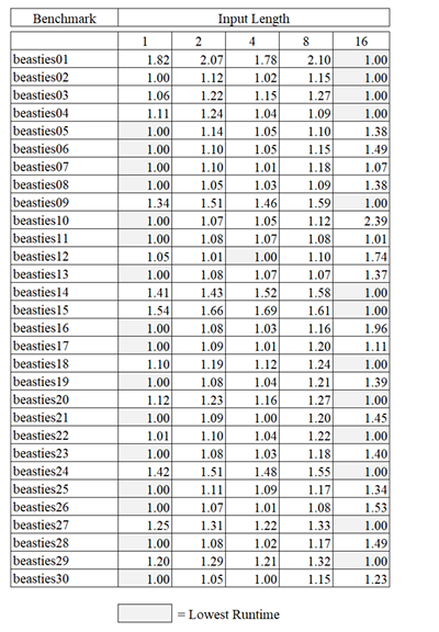

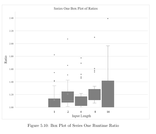

Table 5.5: Benchmark Timings- Series Two
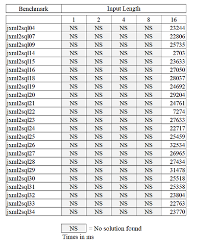

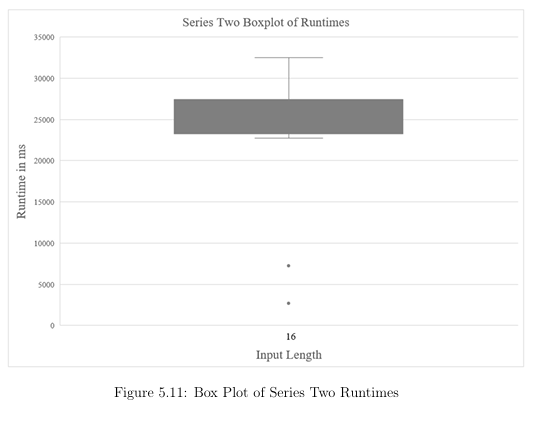

Table 5.6: Benchmark Timings- Series Three
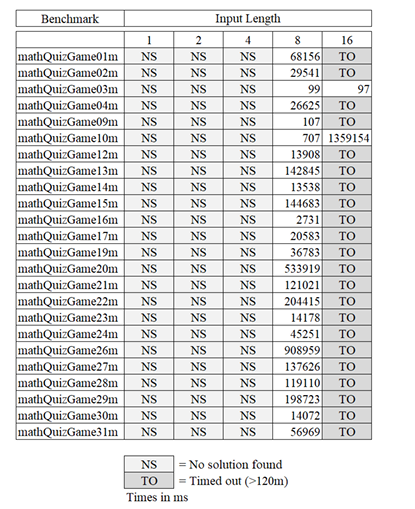

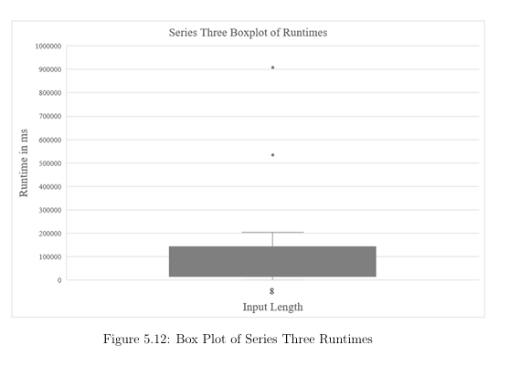

5.3 Scalability
In general, the solution is not scalable since solving string constraints is an undecid able problem [3]. The poor scalability results in the exponential growth in runtime vs. length of string input exhibited by several of the correctness benchmarks in Figure 5.13. However, when applied to real-world benchmarks, the resulting growth with increasing length is not as large, and in the case of benchmark series one, the longest length provided the fastest result in 13 out of 31 benchmarks. The length of the symbolic string inputs is a primary factor in performance degradation, and thus scalability. All string operations in the solver operate on acyclic-automata. These automata are made up of states and transitions. As the length increases, so do the number of states and transitions in the underlying automata. And unlike und bounded or bounded-automata, acyclic-automata re quire at least one additional state and transition for each additional character of input. Thus, as length increases, so do the number of states and transitions that an operation must manipulate, leading to an increase in runtime.
Alphabet size is also a primary determinant in runtime. As the size of the alphabet increases, so do the number of transitions in the underlying automata, and the number of possible values for a given length increases with each additional alphabet symbol. Given an alphabet of size a and a length of symbolic input k the number of possible string values is ak. This becomes problematic when the solver must find consistency in related values. Since the solver iteratively propagates single related value pairs, an increase the number of available pairs has a direct impact on runtime.
It may be possible to restrict the alphabet to only those symbols needed to sat-

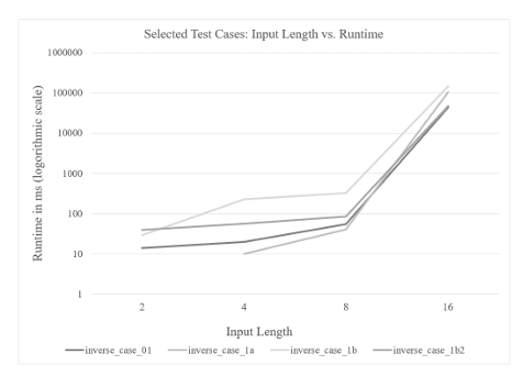
isfy path conditions. In particular, this would be of benefit when handling related values, as the solver would have fewer related pairs to generate and propagate. Table 5.7 shows the effect of adding a single uppercase and lowercase digit to the alphabet of test case 10ab. It is clear that limiting the alphabet to only those values necessary could improve the scalability of the solver.
Table 5.7: Effect of Alphabet Size on Test Case 10ab
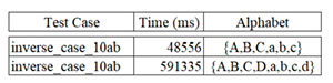

5.4 Validity
There are several factors which may impact the external validity of this evaluation. Restricted Alphabets Since runtime increases quadratically with increases in alphabet size, restricted alphabets are chosen as a default. Table 5.7 demonstrates runtimes quickly become large enough to make the evaluation impractical for certain test cases. However, extending the alphabet in test case 10ab does not affect the solution, only the time taken to achieve it.
Restricted Lengths Since runtime worsens with the increase in length, only experiments with lengths 1, 2, 4, 8 and 16 are evaluated. These appear to be adequate because the solver found solutions for synthetic and real-world bench marks with at least one of these lengths. Further, once a length provides a feasible solution, longer lengths continue that trend. This would tend to indicate that once a minimum length has been determined, testing at longer lengths is unnecessary other than to provide additional analysis data or inputs of greater length.
Inability to Verify Solutions on Real-World Benchmarks The real-world bench marks contained string operations that are not currently supported in SPF. There fore the full testing sequence could not be performed on them at this time. This means we rely on the correctness benchmarks only to verify the correctness of the solver.
5.5 Summary
Experiments answer the research question of whether or not the solver is practical and effective. Data shows that the solver is practical because it finds string inputs for real-world programs benchmarks. The only circumstances in which the solver reports finding no solution are those in which the specified input length is too restrictive. Since the solver successfully generated solutions for real-world programs, it can be said that the solver is effective as well as practical.
The synthetic benchmarks proved to be a greater challenge than many of the benchmarks obtained from real-world programs. This suggests that the solver per formance bottlenecks identified by the synthetic benchmarks may not be prevalent in real-world programs.
SECTION 6
CONCLUSION
This work demonstrates that an automata-based solver can be implemented for generating test inputs for real-world programs, both practically and efficiently. Symbolic Execution was examined in detail, along with possible automata types suitable for representing symbolic strings. Analysis shows the acyclic automata most suitable for our purposes. Novel inverse string operations on automata are presented which guarantee sound and complete results for a given string bound. In cases where the relationship between values must be maintained, this work demonstrates a novel method for ensuring them while keeping the automata model simple. Finally, the analysis of benchmark results shows that the solver is capable of producing correct results in the presence of non-injective and related-value string operations contained in real-world programs.
Future work should focus on the scalability of the solver. The solver currently generates input solutions based on a specified input length. This design choice is based on the need to have a finite input length in order to obtain solutions in a reasonable amount of time. However, as a practical matter, the length of inputs are generally not specified in Java programs other than they must be valid Java strings. Input solutions generated with smaller input sizes that reach a given location during program execution are as viable and usefull as those generated with longer input lengths.
Therefore, it may be beneficial to add a length decision heuristic in which the solver attempts to find a minimum length before starting, perhaps by examining predicate arguments and existing string operations in the constraint graph before starting forward analysis. It could then increase length incrementally in those cases where the chosen input length proves too restrictive to generate a solution. Currently the solver is given an alphabet specification as part of the input. Since alphabet size is a significant factor in runtime, it may be beneficial to have an alphabet determination heuristic that determines a minimum viable alphabet based on the symbols found in concrete and argument values present in the con straint graph. Finally, the solver cannot reliably process related predicates, such as embedded “If” statements. The algorithm should be extended to handle these conditions, possibly utilizing a breadth-first traversal of the TCG instead of depth-first.
REFERENCES
[1] A. Aydin, M. Alkhalaf, and T. Bultan. Automated test generation from
vulnerability signatures. In 2014 IEEE Seventh International Conference on
Software Testing, Verification and Validation, pages 193–202, 2014.
[2] Clark Barrett, Pascal Fontaine, and Cesare Tinelli. The Satisfiability Modulo
Theories Library (SMT-LIB). www.SMT-LIB.org, 2016.
[3] T. Bultan, F. Yu, M. Alkhalaf, and A. Aydin. String Analysis for Software
Verification and Security. Springer International Publishing, AG, 01 2018.
[4] Aske Simon Christensen, Anders Møller, and Michael I. Schwartzbach. Pre
cise analysis of string expressions. In Proceedings of the 10th International
Conference on Static Analysis, SAS’03, page 1–18, Berlin, Heidelberg, 2003.
Springer-Verlag.
[5] L. A. Clarke. A system to generate test data and symbolically execute
programs. IEEE Transactions on Software Engineering, SE-2(3):215–222,
1976.
[6] M. Fujita, P. C. McGeer, and J. C.-Y. Yang. Multi-terminal binary deci
sion diagrams: An efficient datastructure for matrix representation. Form.
Methods Syst. Des., 10(2–3):149–169, April 1997.
[7] I. Ghosh, N. Shafiei, G. Li, and W. Chiang. Jst: An automatic test generation
tool for industrial java applications with strings. In 2013 35th International
Conference on Software Engineering (ICSE), pages 992–1001, 2013.
[8] A. Harris. Suitability of finite state automata to model string constraints in
probabilistic symbolic execution. Boise State University Theses and Disser
tations, 2019.
[9] Pieter Hooimeijer and Margus Veanes. An evaluation of automata algorithms
for string analysis. In Proceedings of the 12th International Conference on
Verification, Model Checking, and Abstract Interpretation, VMCAI’11, page
248–262, Berlin, Heidelberg, 2011. Springer-Verlag.
[10] Scott Kausler and Elena Sherman. Evaluation of string constraint solvers in
the context of symbolic execution. In Proceedings of the 29th ACM/IEEE
International Conference on Automated Software Engineering, ASE ’14, page
259–270, New York, NY, USA, 2014. Association for Computing Machinery.
[11] Adam Kiezun, Vijay Ganesh, Shay Artzi, Philip J. Guo, Pieter Hooimeijer,
and Michael D. Ernst. Hampi: A solver for string constraints. 21(4), February
2013.
[12] James C. King. Symbolic execution and program testing. Commun. ACM,
19(7):385–394, July 1976.
[13] Nils Klarlund and Anders Møller. MONA Version 1.4 User Manual. BRICS,
Department of Computer Science, University of Aarhus, January 2001. Notes
Series NS-01-1. Available from http://www.brics.dk/mona/.
[14] Tianyi Liang, Andrew Reynolds, Nestan Tsiskaridze, Cesare Tinelli, Clark
Barrett, and Morgan Deters. An efficient smt solver for string constraints.
Form. Methods Syst. Des., 48(3):206–234, June 2016.
[15] Gideon Redelinghuys, Willem Visser, and Jaco Geldenhuys. Symbolic execu
tion of programs with strings. In Proceedings of the South African Institute
for Computer Scientists and Information Technologists Conference, SAICSIT
’12, page 139–148, New York, NY, USA, 2012. Association for Computing
Machinery.
[16] E. Sherman and A. Harris. Accurate string constraints solution counting with
weighted automata. In 2019 34th IEEE/ACM International Conference on
Automated Software Engineering (ASE), pages 440–452, 2019.
[17] Willem Visser, Corina S. Păsăreanu, and Sarfraz Khurshid. Test input
generation with java pathfinder. SIGSOFT Softw. Eng. Notes, 29(4):97–107,
July 2004.
[18] F. Yu, T. Bultan, and O.H. Ibarra. Relational string verification using multi
track automata. International Journal of Foundations of Computer Science,
22, 04 2012.
[19] Fang Yu, Muath Alkhalaf, and Tevfik Bultan. Generating vulnerability
signatures for string manipulating programs using automata-based forward
and backward symbolic analyses. In Proceedings of the 2009 IEEE/ACM
International Conference on Automated Software Engineering, ASE ’09, page
605–609, USA, 2009. IEEE Computer Society.
[20] Fang Yu, Muath Alkhalaf, and Tevfik Bultan. Stranger: An automata-based
string analysis tool for php. In Proceedings of the 16th International Confer
ence on Tools and Algorithms for the Construction and Analysis of Systems,
TACAS’10, page 154–157, Berlin, Heidelberg, 2010. Springer-Verlag.
[21] Fang Yu, Tevfik Bultan, Marco Cova, and Oscar H. Ibarra. Symbolic string
verification: An automata-based approach. In Klaus Havelund, Rupak Ma
jumdar, and Jens Palsberg, editors, Model Checking Software, pages 306–324,
Berlin, Heidelberg, 2008. Springer Berlin Heidelberg.
[22] Fang Yu, Tevfik Bultan, and Oscar H Ibarra. Symbolic string verification:
Combining string analysis and size analysis. In International Conference on
Tools and Algorithms for the Construction and Analysis of Systems, pages
322–336. Springer, 2009.
[23] Yunhui Zheng, Xiangyu Zhang, and Vijay Ganesh. Z3-str: A z3-based string
solver for web application analysis. In Proceedings of the 2013 9th Joint
Meeting on Foundations of Software Engineering, ESEC/FSE 2013, page
114–124, New York, NY, USA, 2013. Association for Computing Machinery.
